Seismic Source Model#
Source typologies#
An OpenQuake engine seismic source input model contains a list of sources belonging to a finite set of possible typologies. Each source type is defined by a set of parameters - called source data - which are used to specify the source geometry and the properties of seismicity occurrence.
Currently the OpenQuake engine supports the following source types:
Sources for modelling distributed seismicity:
Point Source - The elemental source type used to model distributed seismicity. Grid and area sources (described below) are different containers of point sources.
Area Source - So far, the most frequently adopted source type in national and regional PSHA models.
Grid Source - A replacement for area sources admitting spatially variable seismicity occurrence properties.
Fault sources with floating ruptures:
Simple Fault Source - The simplest fault model in the OpenQuake engine. This source is habitually used to describe shallow seismogenic faults.
Complex Fault Source - Often used to model subduction interface sources with a complex geometry.
Fault sources with ruptures always covering the entire fault surface:
Characteristic Fault Source - A typology of source where ruptures always fill the entire fault surface.
Non-Parametric Source - A typology of source representing a collection of ruptures, each with their associated probabilities of 0, 1, 2 … occurrences in the investigation time
Sources for representing individual earthquake ruptures
Planar fault rupture - an individual fault rupture represented as a single rectangular plane
Multi-planar fault rupture - an individual rupture represented as a collection of rectangular planes
Simple fault rupture - an individual fault rupture represented as a simple fault surface
Complex fault rupture - an individual fault rupture represented as a complex fault surface
The OpenQuake engine contains some basic assumptions for the definition of these source typologies:
In the case of area and fault sources, the seismicity is homogeneously distributed over the source;
Seismicity temporal occurrence follows a Poissonian model.
The above sets of sources may be referred to as “parametric” sources, that is to say that the generation of the Earthquake Rupture Forecast is done by the OpenQuake engine based on the parameters of the sources set by the user. In some cases, particularly if the user wishes for the temporal occurrence model to be non-Poissonian (such as the lognormal or Brownian Passage Time models) a different type of behaviour is needed. For this OpenQuake engine supports a Non-Parametric Source in which the Earthquake Rupture Forecast is provided explicitly by the user as a set of ruptures and their corresponding probabilities of occurrence.
Source typologies for modelling distributed seismicity#
Point sources#
Single rupture#
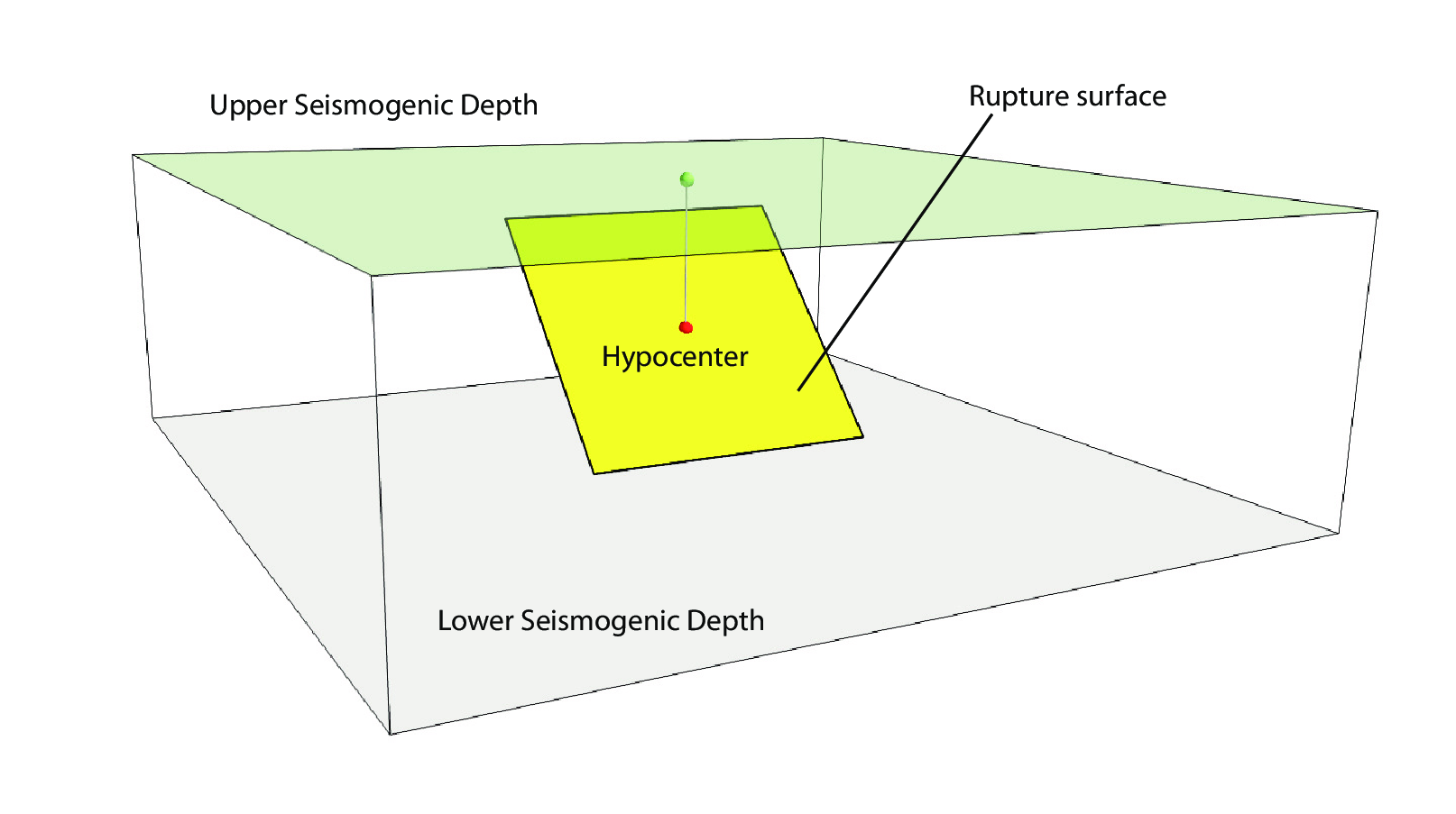
The point source is the elemental source type adopted in the OpenQuake engine for modelling distributed seismicity. The OpenQuake engine always performs calculations considering finite ruptures, even in the case of point sources.
These are the basic assumptions used to generate ruptures with point sources:
Ruptures have a rectangular shape
Rupture hypocenter is located in the middle of the rupture
Ruptures are limited at the top and at the bottom by two planes parallel to the sea level and placed at two characteristic depths named upper and lower seismogenic depths, respectively (see the figure above.)
Source data#
For the definition of a point source the following parameters are required (the figure above shows some of the parameters described below, together with an example of the surface of a generated rupture):
The coordinates of the point (i.e. longitude and latitude) [decimal degrees]
The upper and lower seismogenic depths [km]
One Magnitude-Frequency Distribution
One magnitude-scaling relationship
The rupture aspect ratio
A distribution of nodal planes i.e. one (or several) instances of the following set of parameters:
strike [degrees]
dip [degrees]
rake [degrees]
A magnitude independent depth distribution of hypocenters [km].
The figure below shows ruptures generated by a point source for a range of magnitudes. Each rupture is centered on the single hypocentral position admitted by this point source. Ruptures are created by conserving the area computed using the specified magnitude-area scaling relatioship and the corresponding value of magnitude.
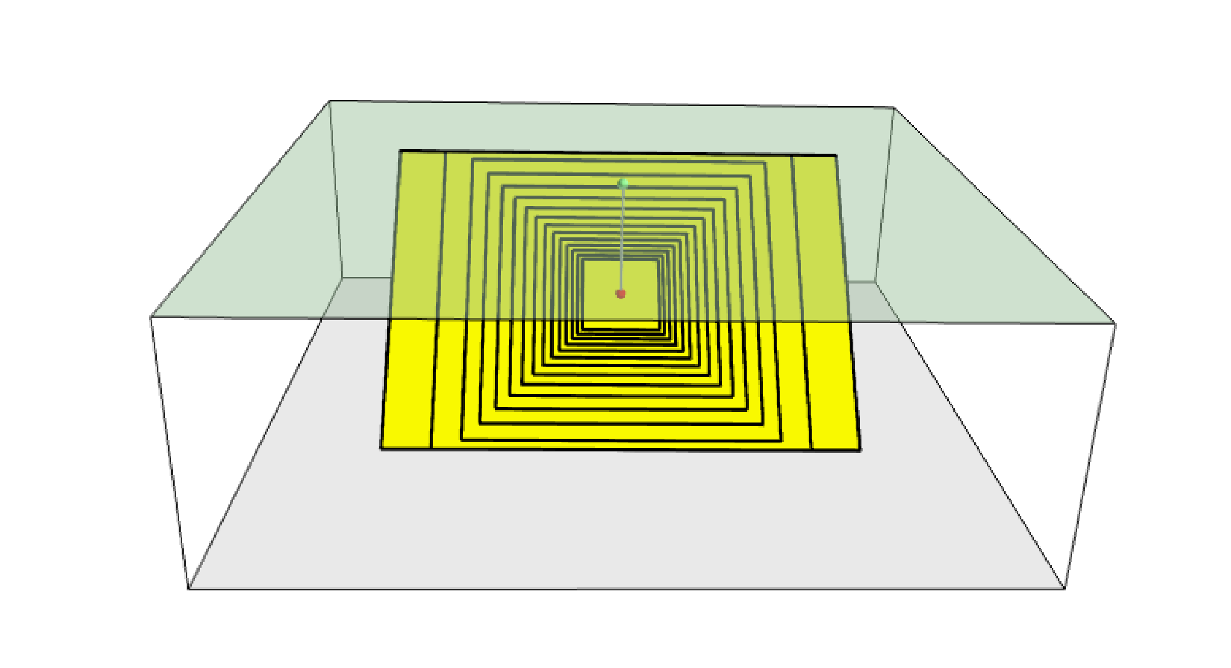
Point source with multiple ruptures. Note the change in the aspect ratio once the rupture width fills the entire seismogenic layer.#
Below we provide the excerpt of an .xml file used to describe the properties of a point source. Note that in this example, ruptures occur on two possible nodal planes and two hypocentral depths. the figure below shows the ruptures generated by the point source.:
<pointSource id="1" name="point" tectonicRegion="Stable Continental Crust">
     <pointGeometry>
         <gml:Point>
             <gml:pos>-122.0 38.0</gml:pos>
         </gml:Point>
         <upperSeismoDepth>0.0</upperSeismoDepth>
         <lowerSeismoDepth>10.0</lowerSeismoDepth>
    </pointGeometry>
    <magScaleRel>WC1994</magScaleRel>
    <ruptAspectRatio>0.5</ruptAspectRatio>
    <truncGutenbergRichterMFD aValue="-3.5" bValue="1.0" minMag="5.0"
                                maxMag="6.5" />
    <nodalPlaneDist>
         <nodalPlane probability="0.3" strike="0.0" dip="90.0" rake="0.0" />
         <nodalPlane probability="0.7" strike="90.0" dip="45.0" rake="90.0" />
    </nodalPlaneDist>
    <hypoDepthDist>
        <hypoDepth probability="0.5" depth="4.0" />
        <hypoDepth probability="0.5" depth="8.0" />
    </hypoDepthDist>
</pointSource>
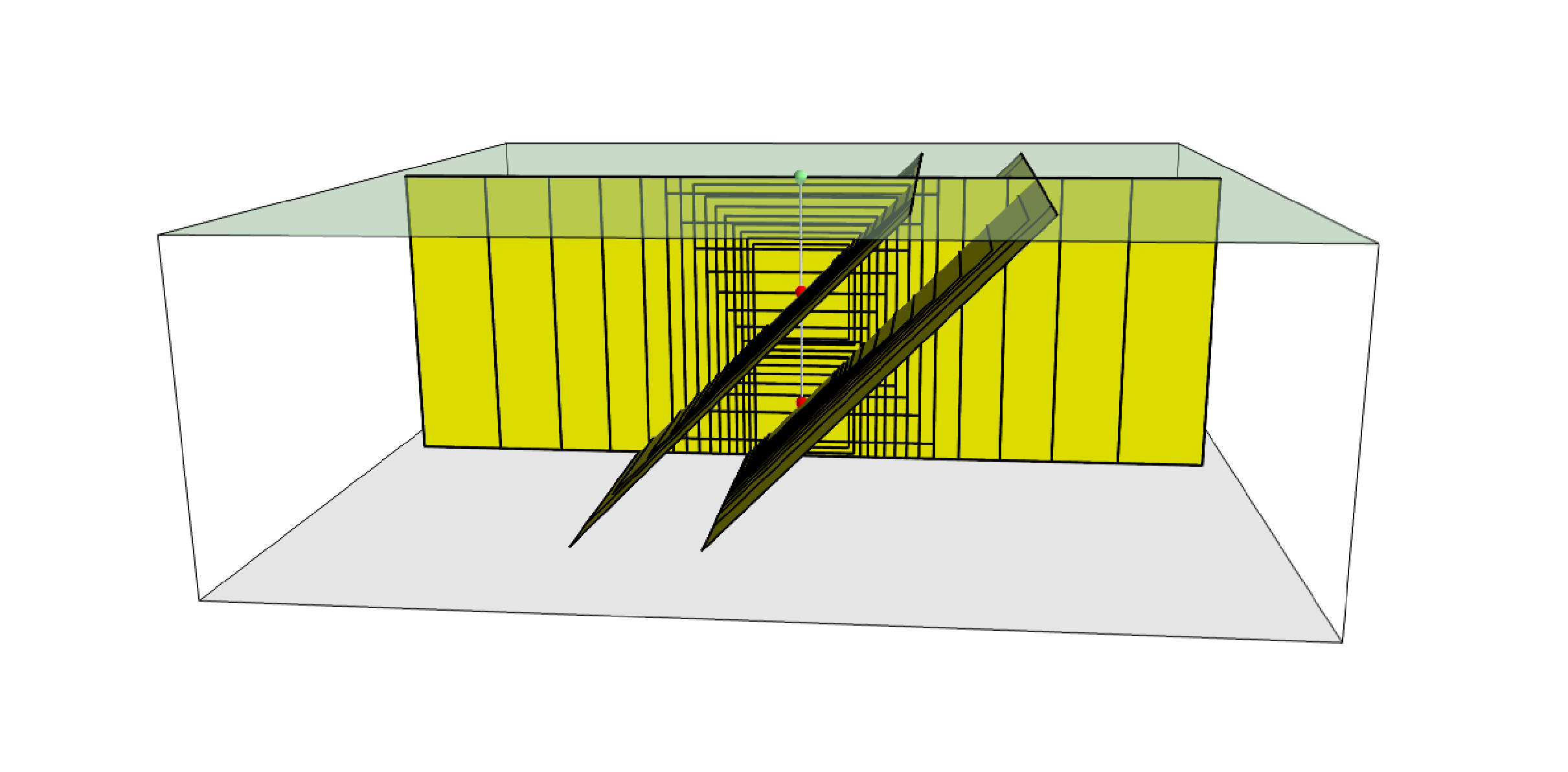
Ruptures produced by the source created using the information in the example .xml file described on page.#
Grid sources#
A Grid Source is simply a collection of point sources distributed over a regular grid (usually equally spaced in longitude and latitude). In Probabilistic Seismic Hazard Analysis a grid source can be considered a model alternative to area sources, since they both model distributed seismicity. Grid sources are generally used to reproduce more faithfully the spatial pattern of seismicity depicted by the earthquakes occurred in the past; in some models (e.g. Petersen et al. (2008)) only events of low and intermediate magnitudes are considered. They are frequently, though not always, computed using seismicity smoothing algorithms (Frankel 1995; Woo 1996, amongst many others).
The use of smoothing algorithms to produce grid sources brings some advantages compared to area sources, since (1) it removes most of the unavoidable degree of subjectivity due to the definition of the geometries of the area sources and (2) it produces a spatial pattern of seismicity that is usually closer to what observed in the reality. Nevertheless, in many cases smoothing algorithms require an a-priori definition of some setup parameters that expose the calculation to a certain degree of partiality.
Grid sources are modeled in OpenQuake engine simply as a set of point sources; in other words, a grid source is just a long list of point sources specified as described in the previous section.
Area sources#
Area sources are usually adopted to describe the seismicity occurring over wide areas where the identification and characterization - i.e. the unambiguous definition of position, geometry and seismicity occurrence parameters - of single fault structures is difficult.
From a computation standpoint, area sources are comparable to grid sources since they are both represented in the engine by a list of point sources.
The OpenQuake engine using the source data parameters (see below) creates an equally spaced in distance grid of point sources where each point has the same seismicity occurrence properties (i.e. rate of events generated).
Below we provide a brief description of the parameters necessary to completely describe an area source.
Source data in area sources#
A polygon defining the external border of the area (i.e. a list of Longitude-Latitude [degrees] tuples) The current version of the OQ-engine doesn’t support the definition of internal borders.
The upper and lower seismogenic depths [km]
One Magnitude-Frequency Distribution
One Magnitude-Scaling Relationship
The rupture aspect ratio
A distribution of nodal planes i.e. one (or several) instances of the following set of parameters
strike [degrees]
dip [degrees]
rake [degrees]
A magnitude independent depth distribution of hypocenters [km].
Below we provide the excerpt of an .xml file used to describe the properties of an area source. The ruptures generated by the area source described in the example are controlled by two nodal planes and have hypocenters at localized at two distinct depths.:
<areaSource id="1" name="Quito" tectonicRegion="Active Shallow Crust">
    <areaGeometry>
      <gml:Polygon>
        <gml:exterior>
          <gml:LinearRing>
            <gml:posList>
              -122.5 37.5
              -121.5 37.5
              -121.5 38.5
              -122.5 38.5
            </gml:posList>
          </gml:LinearRing>
        </gml:exterior>
      </gml:Polygon>
      <upperSeismoDepth>0.0</upperSeismoDepth>
      <lowerSeismoDepth>10.0</lowerSeismoDepth>
    </areaGeometry>
    <magScaleRel>PeerMSR</magScaleRel>
    <ruptAspectRatio>1.5</ruptAspectRatio>
    <incrementalMFD minMag="6.55" binWidth="0.1">
        <occurRates>0.0010614989 8.8291627E-4 7.3437777E-4 6.108288E-4
                    5.080653E-4</occurRates>
    </incrementalMFD>
    <nodalPlaneDist>
        <nodalPlane probability="0.3" strike="0.0" dip="90.0" rake="0.0"/>
        <nodalPlane probability="0.7" strike="90.0" dip="45.0" rake="90.0"/>
    </nodalPlaneDist>
    <hypoDepthDist>
        <hypoDepth probability="0.5" depth="4.0" />
        <hypoDepth probability="0.5" depth="8.0" />
    </hypoDepthDist>
</areaSource>
Fault sources with floating ruptures#
Fault sources in the OpenQuake engine are classified according to the method adopted to distribute ruptures over the fault surface. Two options are currently supported:
With the first option, ruptures with a surface lower than the whole fault surface are floated so as to cover as much as possible homogeneously the fault surface. This model is compatible with all the supported magnitude-frequency distributions.
With the second option, ruptures always fill the entire fault surface. This model is compatible with magnitude-frequency distributions similar to a characteristic model (à la (Schwartz and Coppersmith 1984)).
In this subsection we discuss the different fault source types that support floating ruptures. In the next subsection we will illustrate the fault typology available to model a characteristic rupturing behaviour.
Simple Faults#
Simple Faults are the most common source type used to model shallow faults; the “simple” adjective relates to the geometry description of the source which is obtained by projecting the fault trace (i.e. a polyline) along a characteristic dip direction.
The parameters used to create an instance of this source type are described in the following paragraph.
Source data in simple faults#
A horizontal Fault Trace (usually a polyline). It is a list of longitude-latitude tuples [degrees].
A Frequency-Magnitude Distribution
A Magnitude-Scaling Relationship
A representative value of the dip angle (specified following the Aki-Richards convention; see Aki and Richards (2002)) [degrees]
Rake angle (specified following the Aki-Richards convention; see Aki and Richards (2002)) [degrees]
Upper and lower depth values limiting the seismogenic interval [km]
For near-fault probabilistic seismic hazard analysis, two additional parameters are needed for characterising seismic sources:
A hypocentre list. It is a list of the possible hypocentral positions, and the corresponding weights, e.g., alongStrike=”0.25” downDip=”0.25” weight=”0.25”. Each hypocentral position is defined in relative terms using as a reference the upper left corner of the rupture and by specifying the fraction of rupture length and rupture width.
A slip list. It is a list of the possible rupture slip directions [degrees], and their corresponding weights. The angle describing each slip direction is measured counterclockwise using the fault strike direction as reference.
In near-fault PSHA calculations, the hypocentre list and the slip list are mandatory. The weights in each list must always sum to one. The available GMPE which currently supports the near-fault directivity PSHA calculation in OQ- engine is the ChiouYoungs2014NearFaultEffect GMPE developed by Brian S.-J. Chiou and Youngs (2014) (associated with an Active Shallow Crust tectonic region type).
We provide two examples of simple fault source files. The first is an excerpt of an xml file used to describe the properties of a simple fault source and the second example shows the excerpt of an xml file used to describe the properties of a simple fault source that can be used to perform a PSHA calculation taking into account directivity effects.:
<simpleFaultSource id="1" name="Mount Diablo Thrust"
        tectonicRegion="Active Shallow Crust">
      <simpleFaultGeometry>
          <gml:LineString>
              <gml:posList>
                  -121.82290 37.73010
                  -122.03880 37.87710
              </gml:posList>
          </gml:LineString>
          <dip>45.0</dip>
          <upperSeismoDepth>10.0</upperSeismoDepth>
          <lowerSeismoDepth>20.0</lowerSeismoDepth>
      </simpleFaultGeometry>
      <magScaleRel>WC1994</magScaleRel>
      <ruptAspectRatio>1.5</ruptAspectRatio>
      <incrementalMFD minMag="5.0" binWidth="0.1">
          <occurRates>0.0010614989 8.8291627E-4 7.3437777E-4 6.108288E-4
                      5.080653E-4</occurRates>
      </incrementalMFD>
      <rake>30.0</rake>
      <hypoList>
          <hypo alongStrike="0.25" downDip="0.25" weight="0.25"/>
          <hypo alongStrike="0.25" downDip="0.75" weight="0.25"/>
          <hypo alongStrike="0.75" downDip="0.25" weight="0.25"/>
          <hypo alongStrike="0.75" downDip="0.75" weight="0.25"/>
      </hypoList>
      <slipList>
          <slip weight="0.333">0.0</slip>
          <slip weight="0.333">45.0</slip>
          <slip weight="0.334">90.0</slip>
      </slipList>
</simpleFaultSource>
<simpleFaultSource id="1" name="Mount Diablo Thrust"
        tectonicRegion="Active Shallow Crust">
     <simpleFaultGeometry>
         <gml:LineString>
             <gml:posList>
                 -121.82290 37.73010
                 -122.03880 37.87710
             </gml:posList>
         </gml:LineString>
         <dip>45.0</dip>
         <upperSeismoDepth>10.0</upperSeismoDepth>
         <lowerSeismoDepth>20.0</lowerSeismoDepth>
     </simpleFaultGeometry>
     <magScaleRel>WC1994</magScaleRel>
     <ruptAspectRatio>1.5</ruptAspectRatio>
     <incrementalMFD minMag="5.0" binWidth="0.1">
         <occurRates>0.0010614989 8.8291627E-4 7.3437777E-4 6.108288E-4
                     5.080653E-4</occurRates>
     </incrementalMFD>
     <rake>30.0</rake>
     <hypoList>
         <hypo alongStrike="0.25" downDip="0.25" weight="0.25"/>
         <hypo alongStrike="0.25" downDip="0.75" weight="0.25"/>
         <hypo alongStrike="0.75" downDip="0.25" weight="0.25"/>
         <hypo alongStrike="0.75" downDip="0.75" weight="0.25"/>
     </hypoList>
     <slipList>
         <slip weight="0.333">0.0</slip>
         <slip weight="0.333">45.0</slip>
         <slip weight="0.334">90.0</slip>
     </slipList>
</simpleFaultSource>
Complex Faults#
A complex fault differs from simple fault just by the way the geometry of the fault surface is defined and the fault surface is later created. The input parameters used to describe complex faults are, for the most part, the same used to describe the simple fault typology.
In the case of complex faults, the dip angle is not requested while the fault trace is substituted by two fault edges limiting the top and bottom of the fault surface. Additional curves lying over the fault surface can be specified to complement and refine the description of the fault surface geometry. Unlike the simple fault these edges are not required to be horizontal and may vary in elevation, i.e. the upper edge may represent the intersection between the exposed fault trace and the topographic surface, where positive values indicate below sea level, and negative values indicate above sea level.
Usually, we use complex faults to model intraplate megathrust faults such as the big subduction structures active in the Pacific (Sumatra, South America, Japan) but this source typology can be used also to create - for example - listric fault sources with a realistic geometry.:
<complexFaultSource id="1" name="Cascadia Megathrust"
                    tectonicRegion="Subduction Interface">
    <complexFaultGeometry>
        <faultTopEdge>
            <gml:LineString>
                <gml:posList>
                    -124.704  40.363  0.5493260E+01
                    -124.977  41.214  0.4988560E+01
                    -125.140  42.096  0.4897340E+01
                </gml:posList>
            </gml:LineString>
        </faultTopEdge>
        <intermediateEdge>
            <gml:LineString>
                <gml:posList>
                    -124.704  40.363  0.5593260E+01
                    -124.977  41.214  0.5088560E+01
                    -125.140  42.096  0.4997340E+01
                </gml:posList>
            </gml:LineString>
        </intermediateEdge>
        <intermediateEdge>
            <gml:LineString>
                <gml:posList>
                    -124.704  40.363  0.5693260E+01
                    -124.977  41.214  0.5188560E+01
                    -125.140  42.096  0.5097340E+01
                </gml:posList>
            </gml:LineString>
        </intermediateEdge>
        <faultBottomEdge>
            <gml:LineString>
                <gml:posList>
                    -123.829  40.347  0.2038490E+02
                    -124.137  41.218  0.1741390E+02
                    -124.252  42.115  0.1752740E+02
                </gml:posList>
            </gml:LineString>
        </faultBottomEdge>
    </complexFaultGeometry>
    <magScaleRel>WC1994</magScaleRel>
    <ruptAspectRatio>1.5</ruptAspectRatio>
    <truncGutenbergRichterMFD aValue="-3.5" bValue="1.0" minMag="5.0"
                              maxMag="6.5" />
    <rake>30.0</rake>
</complexFaultSource>
As with the previous examples, the red text highlights the parameters used to specify the source geometry, the parameters in green describe the rupture mechanism, the text in blue describes the magnitude-frequency distribution and the gray text describes the rupture properties.
Fault sources without floating ruptures#
Characteristic faults#
The characteristic fault source is a particular typology of fault created with the assumption that its ruptures will always cover the entire fault surface. As such, no floating is necessary on the surface. The characteristic fault may still take as input a magnitude frequency distribution. In this case, the fault surface can be represented either as a Simple Fault Source surface or as a Complex Fault Source surface or as a combination of rectangular ruptures as represented in the figure below. Mutiple surfaces containing mixed geometry types are also supported.
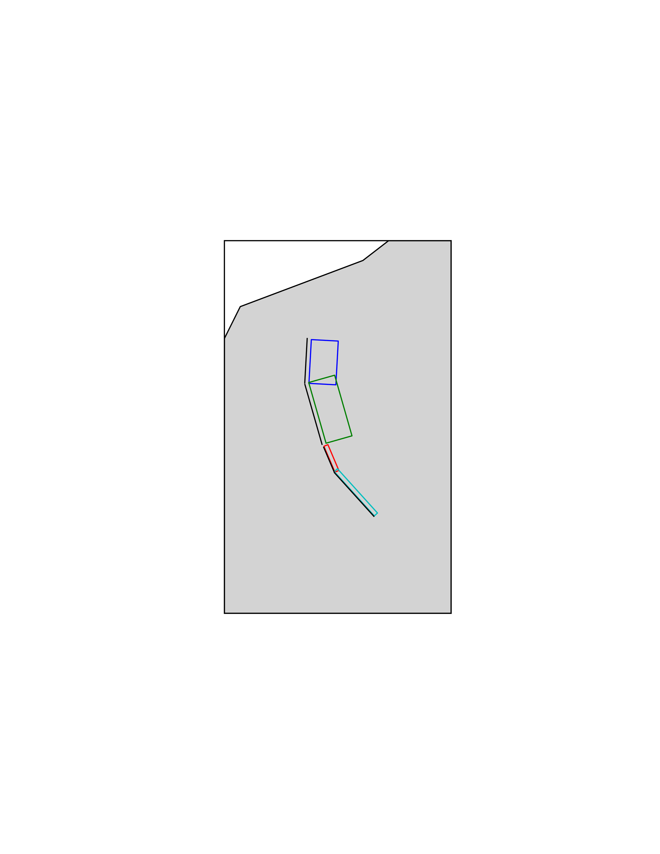
Geometry of a multi-segmented characteristic fault composed of four rectangular ruptures as modelled in OpenQuake engine.#
Source data in characteristic faults#
The characteristic rupture surface is defined through one of the following options:
A list of rectangular ruptures (“planar surfaces”)
A Simple Fault Source geometry
A Complex Fault Source geometry
A Frequency-Magnitude Distribution.
Rake angle (specified following the Aki-Richards convention; see Aki and Richards (2002)).
Upper and lower depth values limiting the seismogenic interval.
A comprehensive example enumerating the possible rupture surface configurations is shown below.:
<characteristicFaultSource id="5" name="characteristic source, simple fault"
                           tectonicRegion="Volcanic">
    <truncGutenbergRichterMFD aValue="-3.5" bValue="1.0"
                              minMag="5.0" maxMag="6.5" />
    <rake>30.0</rake>
    <surface>
        <!-- Characteristic Fault with a simple fault surface -->
        <simpleFaultGeometry>
            <gml:LineString>
                <gml:posList>
                    -121.82290 37.73010
                    -122.03880 37.87710
                </gml:posList>
            </gml:LineString>
            <dip>45.0</dip>
            <upperSeismoDepth>10.0</upperSeismoDepth>
            <lowerSeismoDepth>20.0</lowerSeismoDepth>
        </simpleFaultGeometry>
    </surface>
</characteristicFaultSource>
<characteristicFaultSource id="6" name="characteristic source, complex fault"
                           tectonicRegion="Volcanic">
    <incrementalMFD minMag="5.0" binWidth="0.1">
        <occurRates>0.0010614989 8.8291627E-4 7.3437777E-4</occurRates>
    </incrementalMFD>
    <rake>60.0</rake>
    <surface>
        <!-- Characteristic source with a complex fault surface -->
        <complexFaultGeometry>
            <faultTopEdge>
                <gml:LineString>
                    <gml:posList>
                       -124.704  40.363  0.5493260E+01
                       -124.977  41.214  0.4988560E+01
                       -125.140  42.096  0.4897340E+01
                    </gml:posList>
                </gml:LineString>
            </faultTopEdge>
            <faultBottomEdge>
                <gml:LineString>
                    <gml:posList>
                        -123.829  40.347  0.2038490E+02
                        -124.137  41.218  0.1741390E+02
                        -124.252  42.115  0.1752740E+02
                    </gml:posList>
                </gml:LineString>
            </faultBottomEdge>
        </complexFaultGeometry>
    </surface>
</characteristicFaultSource>
<characteristicFaultSource id="7" name="characteristic source, multi surface"
                           tectonicRegion="Volcanic">
    <truncGutenbergRichterMFD aValue="-3.6" bValue="1.0"
                              minMag="5.2" maxMag="6.4" />
    <rake>90.0</rake>
    <surface>
        <!-- Characteristic source with a collection of planar surfaces -->
        <planarSurface>
            <topLeft lon="-1.0" lat="1.0" depth="21.0" />
            <topRight lon="1.0" lat="1.0" depth="21.0" />
            <bottomLeft lon="-1.0" lat="-1.0" depth="59.0" />
            <bottomRight lon="1.0" lat="-1.0" depth="59.0" />
        </planarSurface>
        <planarSurface strike="20.0" dip="45.0">
             <topLeft lon="1.0" lat="1.0" depth="20.0" />
             <topRight lon="3.0" lat="1.0" depth="20.0" />
             <bottomLeft lon="1.0" lat="-1.0" depth="80.0" />
             <bottomRight lon="3.0" lat="-1.0" depth="80.0" />
         </planarSurface>
    </surface>
</characteristicFaultSource>
Non-Parametric Sources#
Non-Parametric Fault#
The non-parametric fault typology requires that the user indicates the rupture properties (rupture surface, magnitude, rake and hypocentre) and the corresponding probabilities of the rupture. The probabilities are given as a list of floating point values that correspond to the probabilities of \(0,1,2,......,N\) occurrences of the rupture within the specified investigation time. Note that there is not, at present, any internal check to ensure that the investigation time to which the probabilities refer corresponds to that specified in the configuration file. As the surface of the rupture is set explicitly, no rupture floating occurs, and, as in the case of the characteristic fault source, the rupture surface can be defined as either a single planar rupture, a list of planar ruptures, a Simple Fault Source geometry, a Complex Fault Source geometry, or a combination of different geometries.
Comprehensive examples enumerating the possible configurations are shown below:
<nonParametricSeismicSource id="1" name="A Non Parametric Planar Source"
                            tectonicRegion="Some TRT">
    <singlePlaneRupture probs_occur="0.544 0.456">
        <magnitude>8.3</magnitude>
        <rake>90.0</rake>
        <hypocenter depth="26.101" lat="40.726" lon="143.0"/>
        <planarSurface>
            <topLeft depth="9.0" lat="41.6" lon="143.1"/>
            <topRight depth="9.0" lat="40.2" lon="143.91"/>
            <bottomLeft depth="43.202" lat="41.252" lon="142.07"/>
            <bottomRight depth="43.202" lat="39.852" lon="142.91"/>
        </planarSurface>
    </singlePlaneRupture>
    <multiPlanesRupture probs_occur="0.9244 0.0756">
        <magnitude>6.9</magnitude>
        <rake>0.0</rake>
        <hypocenter depth="7.1423" lat="35.296" lon="139.31"/>
        <planarSurface>
            <topLeft depth="2.0" lat="35.363" lon="139.16"/>
            <topRight depth="2.0" lat="35.394" lon="138.99"/>
            <bottomLeft depth="14.728" lat="35.475" lon="139.19"/>
            <bottomRight depth="14.728" lat="35.505" lon="139.02"/>
        </planarSurface>
        <planarSurface>
            <topLeft depth="2.0" lat="35.169" lon="139.34"/>
            <topRight depth="2.0" lat="35.358" lon="139.17"/>
            <bottomLeft depth="12.285" lat="35.234" lon="139.45"/>
            <bottomRight depth="12.285" lat="35.423" lon="139.28"/>
        </planarSurface>
    </multiPlanesRupture>
</nonParametricSeismicSource>
<nonParametricSeismicSource id="2" name="A Non Parametric (Simple) Source"
                            tectonicRegion="Some TRT">
    <simpleFaultRupture probs_occur="0.157 0.843">
        <magnitude>7.8</magnitude>
        <rake>90.0</rake>
        <hypocenter depth="22.341" lat="43.624" lon="147.94"/>
        <simpleFaultGeometry>
            <gml:LineString>
                <gml:posList>
                    147.96 43.202
                    148.38 43.438
                    148.51 43.507
                    148.68 43.603
                    148.76 43.640
                </gml:posList>
            </gml:LineString>
            <dip>30.0</dip>
            <upperSeismoDepth>14.5</upperSeismoDepth>
            <lowerSeismoDepth>35.5</lowerSeismoDepth>
        </simpleFaultGeometry>
    </simpleFaultRupture>
</nonParametricSeismicSource>
<nonParametricSeismicSource id="3" name="A Non Parametric (Complex) Source"
                            tectonicRegion="Some TRT">
    <complexFaultRupture probs_occur="0.157 0.843">
        <magnitude>7.8</magnitude>
        <rake>90.0</rake>
        <hypocenter depth="22.341" lat="43.624" lon="147.94"/>
        <complexFaultGeometry>
            <faultTopEdge>
                <gml:LineString>
                    <gml:posList>
                        148.76 43.64 5.0
                        148.68 43.603 5.0
                        148.51 43.507 5.0
                        148.38 43.438 5.0
                        147.96 43.202 5.0
                    </gml:posList>
                </gml:LineString>
            </faultTopEdge>
            <faultBottomEdge>
               <gml:LineString>
                    <gml:posList>
                        147.92 44.002 35.5
                        147.81 43.946 35.5
                        147.71 43.897 35.5
                        147.5 43.803 35.5
                        147.36 43.727 35.5
                    </gml:posList>
                </gml:LineString>
            </faultBottomEdge>
        </complexFaultGeometry>
    </complexFaultRupture>
</nonParametricSeismicSource>
Magnitude-frequency distributions#
The magnitude-frequency distributions currently supported by the OpenQuake engine are the following:
- A discrete incremental magnitude-frequency distribution
It is the simplest distribution supported. It is defined by the minimum value of magnitude (representing the mid point of the first bin) and the bin width. The distribution itself is simply a sequence of floats describing the annual number of events for different bins. The maximum magnitude admitted by this magnitude-frequency distribution is just the sum of the minimum magnitude and the product of the bin width by the number annual rate values. Below we provide an example of the xml that should be incorporated in a seismic source description in order to define this Magnitude- Frequency Distribution.:
<incrementalMFD minMag="5.05" binWidth="0.1">
    <occurRates>0.15 0.08 0.05 0.03 0.015</occurRates>
</incrementalMFD>
The magnitude-frequency distribution obtained with the above parameters is represented in the figure below.
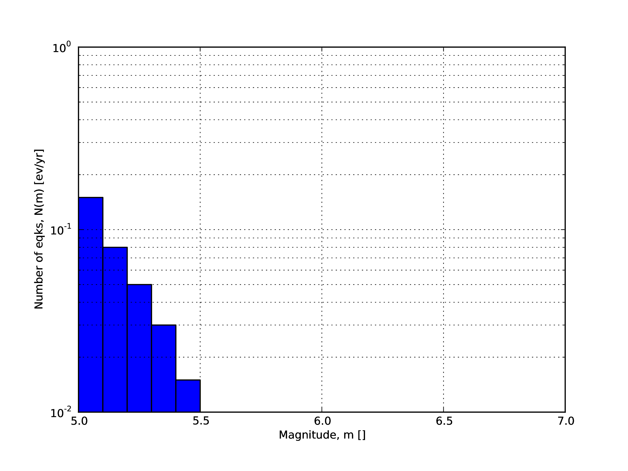
Example of an incremental magnitude-frequency distribution.#
- A double truncated Gutenberg-Richter distribution
This distribution is described by means of a minimum
minMagand maximum magnitudemaxMagand by the :math: a and :math: b values of the Gutenberg-Richter relationship.The syntax of the xml used to describe this magnitude-frequency distribution is rather compact as demonstrated in the following example:
<truncGutenbergRichterMFD aValue="5.0" bValue="1.0" minMag="5.0"
                          maxMag="6.0"/>
The figure below shows the magnitude-frequency distribution obtained using the parameters of the considered example.
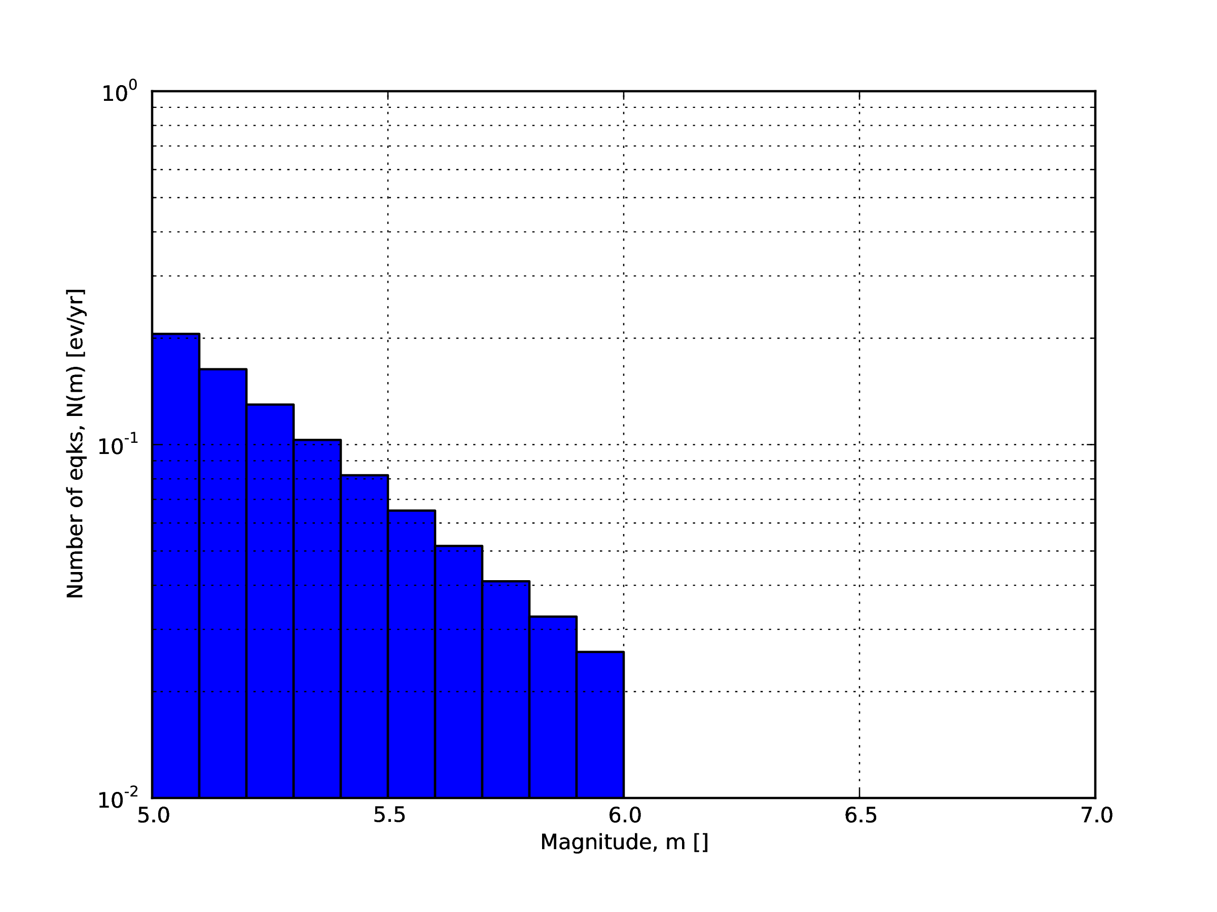
Example of a double truncated Gutenberg-Richter magnitude-frequency distribution.#
- Hybrid Characteristic earthquake model (à la (Youngs and Coppersmith 1985))
The hybrid characteristic earthquake model, presented by (Youngs and Coppersmith 1985), distributes seismic moment proportionally between a characteristic model (for larger magnitudes) and an exponential model. The rate of events is dependent on the magnitude of the characteristic earthquake, the b-value and the total moment rate of the system (:ref:` the figure below <yc-mfd-char-rate>`). However, the total moment rate may be defined in one of two ways. If the total moment rate of the source is known, as may be the case for a fault surface with known area and slip rate, then the distribution can be defined from the total moment rate (in N-m) of the source directly. Alternatively, the distribution can be defined from the rate of earthquakes in the characteristic bin, which may be preferable if the distribution is determined from observed seismicity behaviour. The option to define the distribution according to the total moment rate is input as:
<YoungsCoppersmithMFD minmag="5.0" bValue="1.0" binWidth="0.1"
                      characteristicMag="7.0" totalMomentRate="1.05E19"/>
whereas the option to define the distribution from the rate of the characteristic events is given as:
<YoungsCoppersmithMFD minmag="5.0" bValue="1.0" binWidth="0.1"
                      characteristicMag="7.0" characteristicRate="0.005"/>
Note that in this distribution the width of the magnitude bin must be defined explicitly in the model.
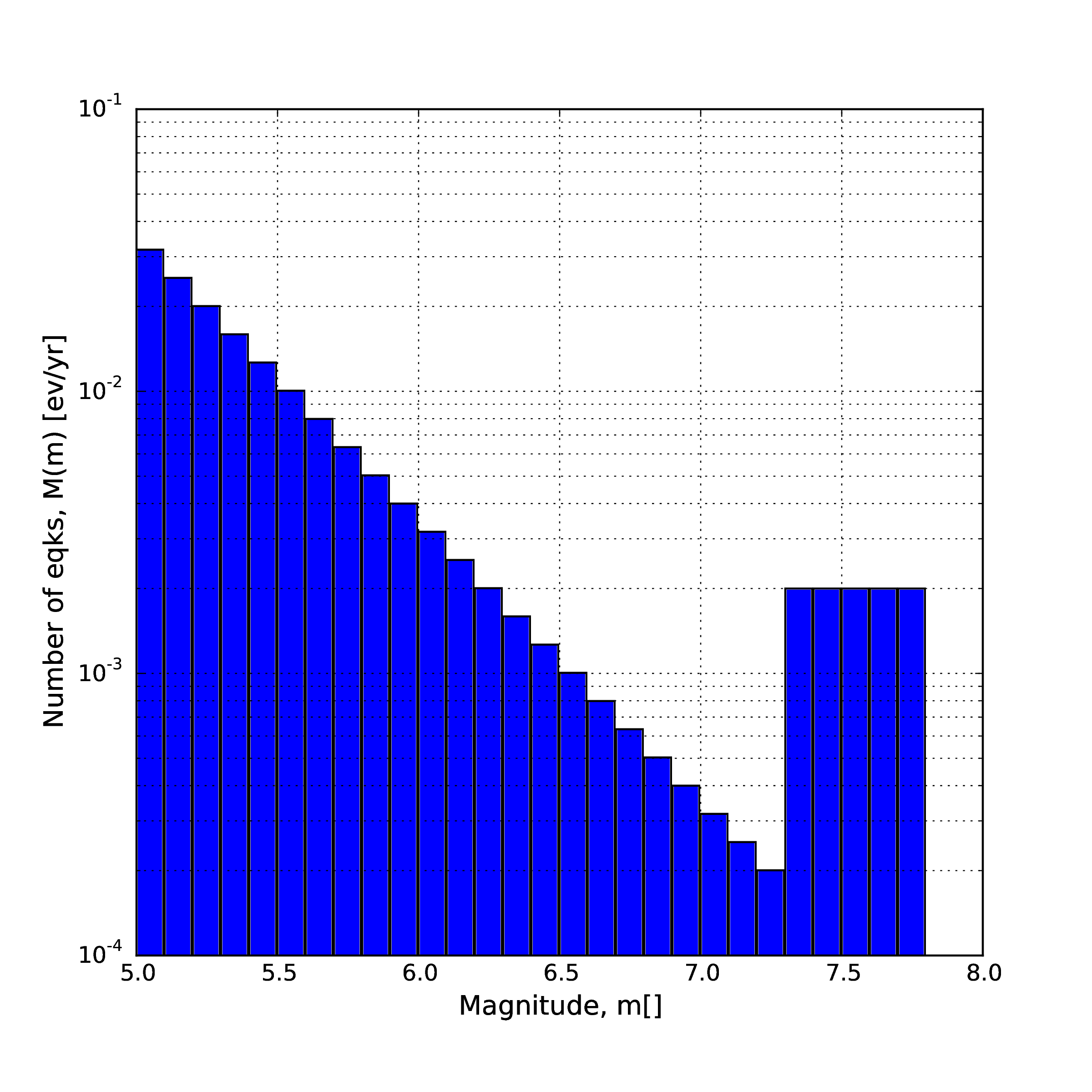
(Youngs and Coppersmith 1985) magnitude-frequency distribution.#
- “Arbitrary” Magnitude Frequency Distribution
The arbitrary magnitude frequency distribution is another non-parametric form of MFD, in which the rates are defined explicitly. Here, the magnitude frequency distribution is defined by a list of magnitudes and their corresponding rates of occurrence. There is no bin-width as the rates correspond exactly to the specific magnitude. Unlike the evenly discretised MFD, there is no requirement that the magnitudes be equally spaced. This distribution (illustrated in the figure below) can be input as:
<arbitraryMFD>
    <occurRates>0.12 0.036 0.067 0.2</occurRates>
    <magnitudes>8.1 8.47 8.68 9.02</magnitude>
</arbitraryMFD>

“Arbitrary” magnitude-frequency distribution.#
Magnitude-scaling relationships#
We provide below a list of the magnitude-area scaling relationships implemented in the OpenQuake engine hazard library (oq-hazardlib):
Relationships for shallow earthquakes in active tectonic regions#
(Wells and Coppersmith 1994) - One of the most well known magnitude scaling relationships, based on a global database of historical earthquake ruptures. The implemented relationship is the one linking magnitude to rupture area, and is called with the keyword
WC1994
Magnitude-scaling relationships for subduction earthquakes#
(Strasser, Arango, and Bommer 2010) - Defines several magnitude scaling relationships for interface and in-slab earthquakes. Only the magnitude to rupture-area scaling relationships are implemented here, and are called with the keywords
StrasserInterfaceandStrasserIntraslabrespectively.(Thingbaijam, Mai, and Goda 2017) - Define magnitude scaling relationships for interface. Only the magnitude to rupture-area scaling relationships are implemented here, and are called with the keywords
ThingbaijamInterface.
Magnitude-scaling relationships stable continental regions#
(EPRI 2011) - Defines a single magnitude to rupture-area scaling relationship for use in the central and eastern United States: \(Area = 10.0^{M_w-4.336}\). It is called with the keyword
CEUS2011
Miscellaneous Magnitude-Scaling Relationships#
PeerMSRdefines a simple magnitude scaling relation used as part of the Pacific Earthquake Engineering Research Center verification of probabilistic seismic hazard analysis programs: \(Area = 10.0^{M_w-4.0}\).PointMSRapproximates a ‘point’ source by returning an infinitesimally small area for all magnitudes. Should only be used for distributed seismicity sources and not for fault sources.
MultiPointSources#
Starting from version 2.5, the OpenQuake engine is able to manage MultiPointSources, i.e. collections of point sources with specific properties. A MultiPointSource is determined by a mesh of points, a MultiMFD magnitude-frequency- distribution and 9 other parameters:
tectonic region type
rupture mesh spacing
magnitude-scaling relationship
rupture aspect ratio
temporal occurrence model
upper seismogenic depth
lower seismogenic depth
NodalPlaneDistribution
HypoDepthDistribution
The MultiMFD magnitude-frequency-distribution is a collection of regular MFD instances (one per point); in order to instantiate a MultiMFD object you need to pass a string describing the kind of underlying MFD (‘arbitraryMFD’, ‘incrementalMFD’, ‘truncGutenbergRichterMFD’ or ‘YoungsCoppersmithMFD’), a float determining the magnitude bin width and few arrays describing the parameters of the underlying MFDs. For instance, in the case of an ‘incrementalMFD’, the parameters are min_mag and occurRates and a MultiMFD object can be instantiated as follows:
mmfd = MultiMFD('incrementalMFD',
              size=2,
              bin_width=[2.0, 2.0],
              min_mag=[4.5, 4.5],
              occurRates=[[.3, .1], [.4, .2, .1]])
In this example there are two points and two underlying MFDs; the occurrence rates can be different for different MFDs: here the first one has 2 occurrence rates while the second one has 3 occurrence rates.
Having instantiated the MultiMFD, a MultiPointSource can be instantiated as in this example:
npd = PMF([(0.5, NodalPlane(1, 20, 3)),
          (0.5, NodalPlane(2, 2, 4))])
hd = PMF([(1, 4)])
mesh = Mesh(numpy.array([0, 1]), numpy.array([0.5, 1]))
tom = PoissonTOM(50.)
rms = 2.0
rar = 1.0
usd = 10
lsd = 20
mps = MultiPointSource('mp1', 'multi point source',
                       'Active Shallow Crust',
                        mmfd, rms, PeerMSR(), rar,
                        tom, usd, lsd, npd, hd, mesh)
There are two major advantages when using MultiPointSources:
the space used is a lot less than the space needed for an equivalent set of PointSources (less memory, less data transfer)
the XML serialization of a MultiPointSource is a lot more efficient (say 10 times less disk space, and faster read/write times)
At computation time MultiPointSources are split into PointSources and are indistinguishable from those. The serialization is the same as for other source typologies (call write_source_model(fname, [mps]) or nrml.to_python(fname, sourceconverter)) and in XML a multiPointSource looks like this:
<multiPointSource
id="mp1"
name="multi point source"
tectonicRegion="Stable Continental Crust"
>
    <multiPointGeometry>
        <gml:posList>
            0.0 1.0 0.5 1.0
        </gml:posList>
        <upperSeismoDepth>
            10.0
        </upperSeismoDepth>
        <lowerSeismoDepth>
            20.0
        </lowerSeismoDepth>
    </multiPointGeometry>
    <magScaleRel>
        PeerMSR
    </magScaleRel>
    <ruptAspectRatio>
        1.0
    </ruptAspectRatio>
    <multiMFD
    kind="incrementalMFD"
    size=2
    >
        <bin_width>
            2.0 2.0
        </bin_width>
        <min_mag>
            4.5 4.5
        </min_mag>
        <occurRates>
            0.10 0.05 0.40 0.20 0.10
        </occurRates>
        <lengths>
            2 3
        </lengths>
    </multiMFD>
    <nodalPlaneDist>
        <nodalPlane dip="20.0" probability="0.5" rake="3.0" strike="1.0"/>
        <nodalPlane dip="2.0" probability="0.5" rake="4.0" strike="2.0"/>
    </nodalPlaneDist>
    <hypoDepthDist>
        <hypoDepth depth="14.0" probability="1.0"/>
    </hypoDepthDist>
</multiPointSource>
The node <lengths> contains the lengths of the occurrence rates, 2 and 3 respectively in this example. This is needed since the serializer writes the occurrence rates sequentially (in this example they are the 5 floats 0.10 0.05 0.40 0.20 0.10) and the information about their grouping would be lost otherwise.
There is an optimization for the case of homogeneous parameters; for instance in this example the bin_width and min_mag are the same in all points; then it is possible to store these as one-element lists:
mmfd = MultiMFD('incrementalMFD',
                size=2,
                bin_width=[2.0],
                min_mag=[4.5],
                occurRates=[[.3, .1], [.4, .2, .1]])
This saves memory and data transfer, compared to the version of the code above.
Notice that writing bin_width=2.0 or min_mag=4.5 would be an error: the parameters must be vector objects; if their length is 1 they are treated as homogeneous vectors of size size. If their length is different from 1 it must be equal to size, otherwise you will get an error at instantiation time.
The point source gridding approximation#
WARNING: the point source gridding approximation is used only in classical calculations, not in event based calculations!
Most hazard calculations are dominated by distributed seismicity, i.e. area sources and multipoint sources that for the engine are just regular point sources. In such situations the parameter governing the performance is the grid spacing: a calculation with a grid spacing of 50 km produces 25 times less ruptures and it is expected to be 25 times faster than a calculation with a grid spacing of 10 km.
The point source gridding approximation is a smart way of raising the grid spacing without losing too much precision and without losing too much performance.
The idea is two use two kinds of point sources: the original ones and a set of “effective” ones (instances of the class
CollapsedPointSource) that essentially are the original sources averaged on a larger grid, determined by the parameter
ps_grid_spacing.
The plot below should give the idea, the points being the original sources and the squares with ~25 sources each being associated to the collapsed sources:
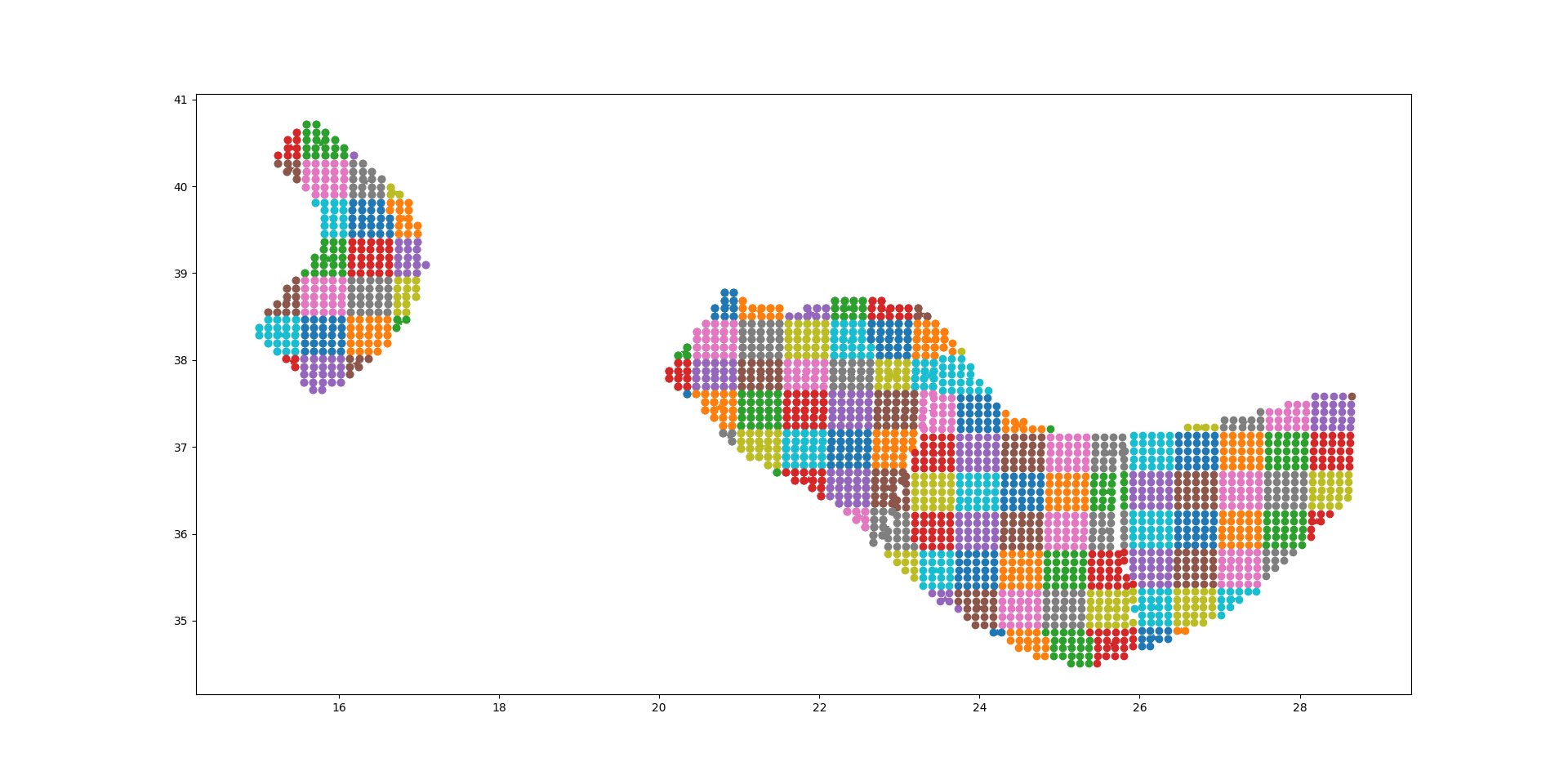
For distant sites it is possible to use the large grid (i.e. the CollapsePointSources) without losing much precision, while for close points the original sources must be used.
The engine uses the parameter pointsource_distance to determine when to use the original sources and when to use
the collapsed sources.
If the maximum_distance has a value of 500 km and the pointsource_distance a value of 50 km, then
(50/500)^2 = 1% of the sites will be close and 99% of the sites will be far. Therefore you will able to use the
collapsed sources for 99% percent of the sites and a huge speedup is to big expected (in reality things are a bit more
complicated, since the engine also consider the fact that ruptures have a finite size, but you get the idea).
Application: making the Canada model 26x faster#
In order to give a concrete example, I ran the Canada 2015 model on 7 cities by using the following site_model.csv file:
custom_site_id |
lon |
lat |
vs30 |
z1pt0 |
z2pt5 |
|---|---|---|---|---|---|
montre |
-73 |
45 |
368 |
393.6006 |
1.391181 |
calgar |
-114 |
51 |
451 |
290.6857 |
1.102391 |
ottawa |
-75 |
45 |
246 |
492.3983 |
2.205382 |
edmont |
-113 |
53 |
372 |
389.0669 |
1.374081 |
toront |
-79 |
43 |
291 |
465.5151 |
1.819785 |
winnip |
-97 |
50 |
229 |
499.7842 |
2.393656 |
vancou |
-123 |
49 |
600 |
125.8340 |
0.795259 |
Notice that we are using a custom_site_id field to identify the cities. This is possible only in engine versions
>= 3.13, where custom_site_id has been extended to accept strings of at most 6 characters, while before only
integers were accepted (we could have used a zip code instead).
If no special approximations are used, the calculation is extremely slow, since the model is extremely large. On the
the GEM cluster (320 cores) it takes over 2 hours to process the 7 cities. The dominating operation, as of engine 3.13,
is “computing mean_std” which takes, in total, 925,777 seconds split across the 320 cores, i.e. around 48 minutes per
core. This is way too much and it would make impossible to run the full model with ~138,000 sites. An analysis shows
that the calculation time is totally dominated by the point sources. Moreover, the engine prints a warning saying that
I should use the pointsource_distance approximation. Let’s do so, i.e. let us set pointsource_distance = 50
in the job.ini file. That alone triples the speed of the engine, and the calculation times in “computing mean_std” goes
down to 324,241 seconds, i.e. 16 minutes per core, in average. An analysis of the hazard curves shows that there is
practically no difference between the original curves and the ones computed with the approximation on:
$ oq compare hcurves PGA <first_calc_id> <second_calc_id>
There are no differences within the tolerances atol=0.001, rtol=0%, sids=[0 1 2 3 4 5 6]
However, this is not enough. We are still too slow to run the full model in a reasonable amount of time. Enters the
point source gridding. By setting ps_grid_spacing=50 we can spectacularly reduce the calculation time to 35,974s,
down by nearly an order of magnitude! This time oq compare hcurves produces some differences on the last city but
they are minor and not affecting the hazard maps:
$ oq compare hmaps PGA <first_calc_id> <third_calc_id>
There are no differences within the tolerances atol=0.001, rtol=0%, sids=[0 1 2 3 4 5 6]
The following table collects the results:
operation |
calc_time |
approx |
speedup |
|---|---|---|---|
computing mean_std |
925_777 |
no approx |
1x |
computing mean_std |
324_241 |
pointsource_distance |
3x |
computing mean_std |
35_974 |
ps_grid_spacing |
26x |
It should be noticed that if you have 130,000 sites it is likely that there will be a few sites where the point source
gridding approximation gives results quite different for the exact results. The commands oq compare allows you to
figure out which are the problematic sites, where they are and how big is the difference from the exact results.
You should take into account that even the “exact” results have uncertainties due to all kind of reasons, so even a large difference can be quite acceptable. In particular if the hazard is very low you can ignore any difference since it will have no impact on the risk.
Points with low hazard are expected to have large differences, this is why by default oq compare use an absolute
tolerance of 0.001g, but you can raise that to 0.01g or more. You can also give a relative tolerance of 10% or more.
Internally oq compare calls the function numpy.allclose see https://numpy.org/doc/stable/reference/generated/numpy.allclose.html
for a description of how the tolerances work.
By increasing the pointsource_distance parameter and decreasing the ps_grid_spacing parameter one can make the
approximation as precise as wanted, at the expense of a larger runtime.
NB: the fact that the Canada model with 7 cities can be made 26 times faster does not mean that the same speedup apply
when you consider the full 130,000+ sites. A test with ps_grid_spacing=pointsource_distance=50 gives a speedup of 7
times, which is still very significant.
How to determine the “right” value for the ps_grid_spacing parameter#
The trick is to run a sensitivity analysis on a reduced calculation. Set in the job.ini something like this:
sensitivity_analysis = {'ps_grid_spacing': [0, 20, 40, 60]}
and then run:
$ OQ_SAMPLE_SITES=.01 oq engine --run job.ini
This will run sequentially 4 calculations with different values of the ps_grid_spacing. The first calculation, the
one with ps_grid_spacing=0, is the exact calculation, with the approximation disabled, to be used as reference.
Notice that setting the environment variable OQ_SAMPLE_SITES=.01 will reduced by 100x the number of sites: this is
essential in order to make the calculation times acceptable in large calculations.
After running the 4 calculations you can compare the times by using oq show performance and the precision by using
oq compare. From that you can determine which value of the ps_grid_spacing gives a good speedup with a decent
precision. Calculations with plenty of nodal planes and hypocenters will benefit from lower values of ps_grid_spacing
while calculations with a single nodal plane and hypocenter for each source will benefit from higher values of
ps_grid_spacing.
If you are interested only in speed and not in precision, you can set calculation_mode=preclassical, run the
sensitivity analysis in parallel very quickly and then use the ps_grid_spacing value corresponding to the minimum
weight of the source model, which can be read from the logs. Here is the trick to run the calculations in parallel:
$ oq engine --multi --run job.ini -p calculation_mode=preclassical
And here is how to extract the weight information, in the example of Alaska, with job IDs in the range 31692-31695:
$ oq db get_weight 31692
<Row(description=Alaska{'ps_grid_spacing': 0}, message=tot_weight=1_929_504, max_weight=120_594, num_sources=150_254)>
$ oq db get_weight 31693
<Row(description=Alaska{'ps_grid_spacing': 20}, message=tot_weight=143_748, max_weight=8_984, num_sources=22_727)>
$ oq db get_weight 31694
<Row(description=Alaska{'ps_grid_spacing': 40}, message=tot_weight=142_564, max_weight=8_910, num_sources=6_245)>
$ oq db get_weight 31695
<Row(description=Alaska{'ps_grid_spacing': 60}, message=tot_weight=211_542, max_weight=13_221, num_sources=3_103)>
The lowest weight is 142_564, corresponding to a ps_grid_spacing of 40km; since the weight is 13.5 times smaller
than the weight for the full calculation (1_929_504), this is the maximum speedup that we can expect from using the
approximation.
Note 1: the weighting algorithm changes at every release, so only relative weights at a fixed release are meaningful and it does not make sense to compare weights across engine releases.
Note 2: the precision and performance of the ps_grid_spacing approximation change at every release: you should not
expect to get the same numbers and performance across releases even if the model is the same and the parameters are the
same.