Logic Trees#
Defining Logic Trees#
The main components of a logic tree structure in the OpenQuake engine are the following:
- Branch:
The simplest component of a logic tree structure. A Branch represent a possible interpretation of a value assignment for a specific type of uncertainty. It is fully described by the tuple (parameter or model, weight).
- Branching set:
It is a key component in the logic tree structure used by the OpenQuake engine. It groups a set of branches i.e. alternative interpretations of a parameter or a model. Each branching set is defined by:
An ID
An uncertainty type (for a comprehensive list of the types of uncertainty currently supported see section Logic trees as described in the nrml schema)
One or more branches
This set of uncertainties can be applied to the whole initial seismic source input model or just to a subset of seismic sources. The sum of the weights/probabilities assigned to the set of branches always correspond to one.
Below we provide a simple schema illustrating the skeleton of xml file containing the desciption of a logic tree:
<logicTreeBranchSet branchSetID=ID
                    uncertaintyType=TYPE>
    <logicTreeBranch>
        <uncertaintyModel>VALUE</uncertaintyModel>
        <uncertaintyWeight>WEIGHT</uncertaintyWeight>
    </logicTreeBranch>
</logicTreeBranchSet>
As it appears from this example, the structure of a logic tree is a set of nested elements.
A schematic representation of the elemental components of a logic tree structure is provided in the figure below. A Branch set identifies a collection of branches (i.e. individual branches) whose weights sum to 1.
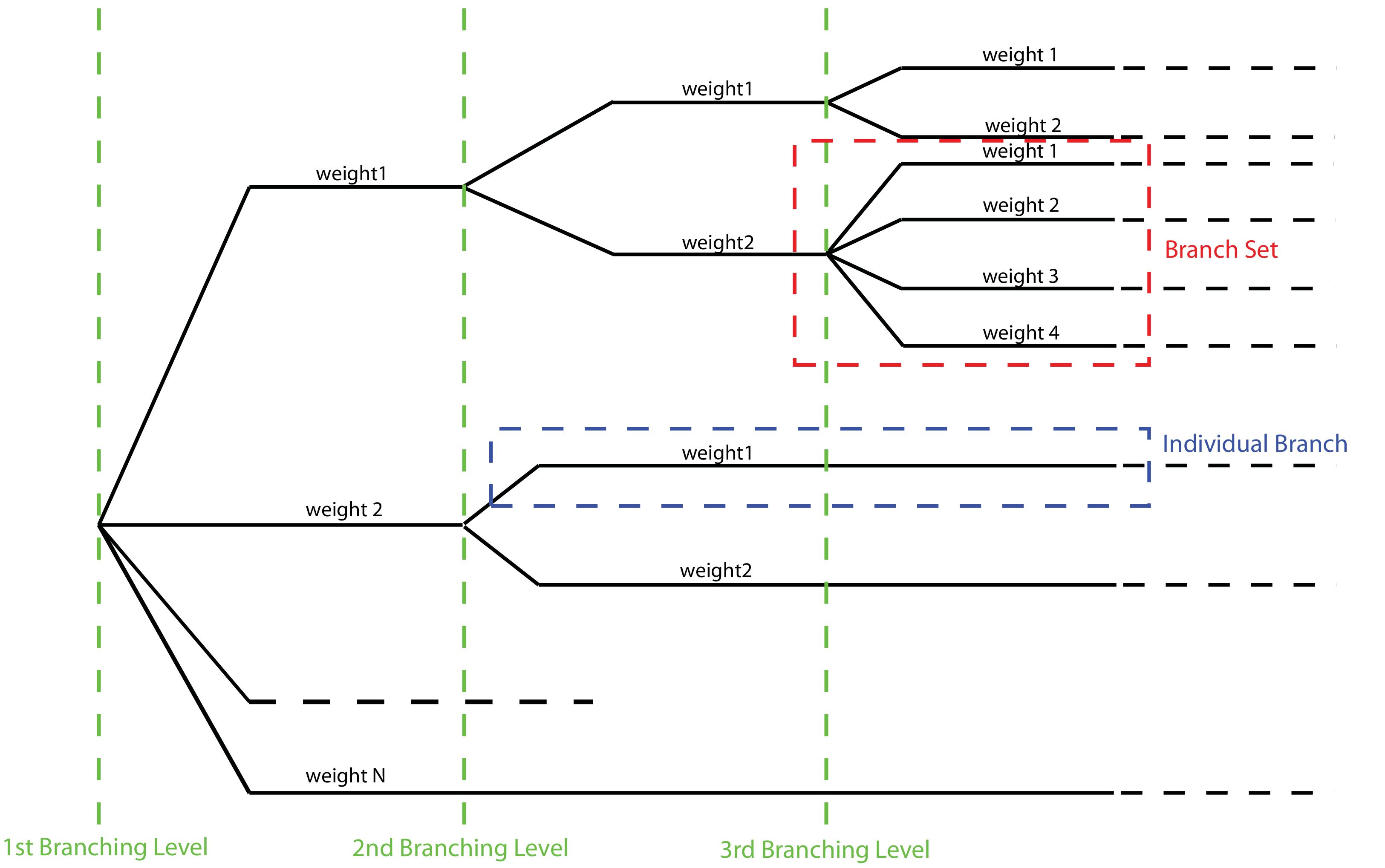
Generic Logic Tree structure as described in terms of Branch sets, and individual branches.#
Logic trees as described in the nrml schema#
In the NRML schema, a logic tree structure is defined through the logicTree element:
<logicTree logicTreeID="ID">
...
</logicTree>
A logicTree contains as a sequence of logicTreeBranchSet elements.
There are no restrictions on the number of Branch set that can be defined.
Each logicTreeBranchSet has two required attributes: branchSetID and uncertaintyType. The latter defines the
type of epistemic uncertainty this Branch set is describing.:
<logicTree logicTreeID="ID">
             <logicTreeBranchSet branchSetID="ID_1"
                     uncertaintyType="UNCERTAINTY_TYPE">
                     ...
             </logicTreeBranchSet>
             <logicTreeBranchSet branchSetID="ID_2"
                     uncertaintyType="UNCERTAINTY_TYPE">
                     ...
             </logicTreeBranchSet>
             ...
             <logicTreeBranchSet branchSetID="ID_N"
                     uncertaintyType="UNCERTAINTY_TYPE">
                     ...
             </logicTreeBranchSet>
...
</logicTree>
Possible values for the uncertaintyType attribute are:
gmpeModel: indicates epistemic uncertainties on ground motion prediction equationssourceModel: indicates epistemic uncertainties on source modelsmaxMagGRRelative: indicates relative (i.e. increments) epistemic uncertainties to be added (or subtracted, depending on the sign of the increment) to the Gutenberg-Richter maximum magnitude value.bGRRelative: indicates relative epistemic uncertainties to be applied to the Gutenberg-Richter b value.abGRAbsolute: indicates absolute (i.e. values used to replace original values) epistemic uncertainties on the Gutenberg-Richter a and b values.maxMagGRAbsolute: indicates (absolute) epistemic uncertainties on the Gutenberg-Richter maximum magnitude.incrementalMFDAbsolute: indicates (absolute) epistemic uncertainties on the incremental magnitude frequency distribution (i.e. alternative rates and/or minimum magnitude) of a specific source (can only be applied to individual sources)simpleFaultGeometryAbsolute: indicates alternative representations of the simple fault geometry for an individual simple fault sourcesimpleFaultDipRelative: indicates a relative increase or decrease in fault dip for one or more simple fault sourcessimpleFaultDipAbsolute: indicates alternative values of fault dip for one or more simple fault sourcescomplexFaultGeometryAbsolute: indicates alternative representations of complex fault geometry for an individual complex fault sourcecharacteristicFaultGeometryAbsolute: indicates alternative representations of the characteristic fault geometry for an individual characteristic fault source
A branchSet is defined as a sequence of logicTreeBranch elements, each specified by an uncertaintyModel
element (a string identifying an uncertainty model; the content of the string varies with the uncertaintyType
attribute value of the branchSet element) and the uncertaintyWeight element (specifying the probability/weight
associated to the uncertaintyModel):
< logicTree  logicTreeID="ID">
...

             < logicTreeBranchSet  branchSetID="ID_#"
                             uncertaintyType="UNCERTAINTY_TYPE">
                     < logicTreeBranch  branchID="ID_1">
                             <uncertaintyModel>
                                 UNCERTAINTY_MODEL
                             </uncertaintyModel>
                             <uncertaintyWeight>
                                 UNCERTAINTY_WEIGHT
                             </uncertaintyWeight>
                     </ logicTreeBranch >
                     ...
                     < logicTreeBranch  branchID="ID_N">
                             <uncertaintyModel>
                                 UNCERTAINTY_MODEL
                             </uncertaintyModel>
                             <uncertaintyWeight>
                                 UNCERTAINTY_WEIGHT
                             </uncertaintyWeight>
                     </logicTreeBranch>
             </logicTreeBranchSet>
...
</logicTree >
Depending on the uncertaintyType the content of the <uncertaintyModel> element changes:
if
uncertaintyType="gmpeModel", the uncertainty model contains the name of a ground motion prediction equation (a list of available GMPEs can be obtained usingoq info gsimsand these are also documented here):<uncertaintyModel>GMPE_NAME</uncertaintyModel>
if
uncertaintyType="sourceModel", the uncertainty model contains the paths to a source model file, e.g.:<uncertaintyModel>SOURCE_MODEL_FILE_PATH</uncertaintyModel>
if
uncertaintyType="maxMagGRRelative", the uncertainty model contains the increment to be added (or subtracted, depending on the sign) to the Gutenberg-Richter maximum magnitude:<uncertaintyModel>MAX_MAGNITUDE_INCREMENT</uncertaintyModel>
if
uncertaintyType="bGRRelative", the uncertainty model contains the increment to be added (or subtracted, depending on the sign) to the Gutenberg-Richter b value:<uncertaintyModel>B_VALUE_INCREMENT</uncertaintyModel>
if
uncertaintyType="abGRAbsolute", the uncertainty model must contain one a and b pair:<uncertaintyModel>A_VALUE B_VALUE</uncertaintyModel>
if
uncertaintyType="maxMagGRAbsolute", the uncertainty model must contain one Gutenberg-Richter maximum magnitude value:<uncertaintyModel>MAX_MAGNITUDE</uncertaintyModel>
if
uncertaintyType="incrementalMFDAbsolute", the uncertainty model must contain an instance of the incremental MFD node:<uncertaintyModel> <incrementalMFD minMag="MIN MAGNITUDE" binWidth="BIN WIDTH"> <occurRates>RATE_1 RATE_2 ... RATE_N</occurRates> </incrementalMFD> </uncertaintyModel>
if
uncertaintyType="simpleFaultGeometryAbsolute"then the uncertainty model must contain a valid instance of thesimpleFaultGeometrynode as described in section Simple Faultsif
uncertaintyType="simpleFaultDipRelative"then the uncertainty model must specify the number of degrees to increase (positive) or decrease (negative) the fault dip. Note that if this increase results in an adjusted fault dip greater than 90 degrees or less than 0 degrees an error will occur.:<uncertaintyModel>DIP_INCREMENT</uncertaintyModel>
if
uncertaintyType="simpleFaultDipAbsolute"then the uncertainty model must specify the dip angle (in degrees):<uncertaintyModel>DIP</uncertaintyModel>
if
uncertaintyType="complexFaultGeometryAbsolute"then the uncertainty model must contain a valid instance of thecomplexFaultGeometrysource node as described in section Complex Faultsif
uncertaintyType="characteristicFaultGeometryAbsolute"then the uncertainty model must contain a valid instance of thecharacteristicFaultGeometrysource node, as described in section Characteristic faults
The maximum number of logicTreeBranch elements per branchset is 182 and the uncertainty weights should sum to 1.0.
The logicTreeBranchSet element offers also a number of optional attributes allowing for complex tree definitions:
applyToBranches: specifies to whichlogicTreeBranchelements (one or more), in the previous Branch sets, the Branch set is linked to. The linking is established by defining the IDs of the branches to link to:applyToBranches="branchID1 branchID2 .... branchIDN"
The default is the keyword ALL, which means that a Branch set is by default linked to all branches in the previous Branch set. By specifying one or more branches to which the Branch set links to, non-symmetric logic trees can be defined.
applyToSources: specifies to which source in a source model the uncertainty applies to. Sources are specified in terms of their IDs:applyToSources="srcID1 srcID2 .... srcIDN"
applyToTectonicRegionType: specifies to which tectonic region type the uncertainty applies to. Only one tectonic region type can be defined (Active Shallow Crust,Stable Shallow Crust,Subduction Interface,Subduction IntraSlab,Volcanic), e.g.:applyToTectonicRegionType=”Active Shallow Crust”
The Seismic Source System#
The Seismic Source System contains the model (or the models) describing position, geometry and activity of seismic sources of engineering importance for a set of sites as well as the possible epistemic uncertainties to be incorporated into the calculation of seismic hazard.
The Seismic Source Logic Tree#
The structure of the Seismic Source Logic Tree consists of at least one Branch Set. The example provided below shows the simplest Seismic Source Logic Tree structure that can be defined in a Psha Input Model for OpenQuake engine. It’s a logic tree with just onebranchset with one Branch used to define the initial seismic source model (its weight will be equal to one).:
<?xml version="1.0" encoding="UTF-8"?>
<nrml xmlns:gml="http://www.opengis.net/gml"
      xmlns="http://openquake.org/xmlns/nrml/0.5">
    <logicTree logicTreeID="lt1">
            <logicTreeBranchSet uncertaintyType="sourceModel"
                                branchSetID="bs1">
                <logicTreeBranch branchID="b1">
                    <uncertaintyModel>seismic_source_model.xml
                    </uncertaintyModel>
                    <uncertaintyWeight>1.0</uncertaintyWeight>
                </logicTreeBranch>
            </logicTreeBranchSet>
    </logicTree>
</nrml>
The optional branching levels will contain rules that modify parameters of the sources in the initial seismic source model.
For example, if the epistemic uncertainties to be considered are source geometry and maximum magnitude, the modeller can create a logic tree structure with three initial seismic source models (each one exploring a different definition of the geometry of sources) and one branching level accounting for the epistemic uncertainty on the maximum magnitude.
Below we provide an example of such logic tree structure. Note that the uncertainty on the maximum magnitude is specified in terms of relative increments with respect to the initial maximum magnitude defined for each source in the initial seismic source models.:
<?xml version="1.0" encoding="UTF-8"?>
<nrml xmlns:gml="http://www.opengis.net/gml"
      xmlns="http://openquake.org/xmlns/nrml/0.5">
    <logicTree logicTreeID="lt1">

            <logicTreeBranchSet uncertaintyType="sourceModel"
                                branchSetID="bs1">
                <logicTreeBranch branchID="b1">
                    <uncertaintyModel>seismic_source_model_A.xml
                    </uncertaintyModel>
                    <uncertaintyWeight>0.2</uncertaintyWeight>
                </logicTreeBranch>
                <logicTreeBranch branchID="b2">
                    <uncertaintyModel>seismic_source_model_B.xml
                    </uncertaintyModel>
                    <uncertaintyWeight>0.3</uncertaintyWeight>
                </logicTreeBranch>
                <logicTreeBranch branchID="b3">
                    <uncertaintyModel>seismic_source_model_C.xml
                    </uncertaintyModel>
                    <uncertaintyWeight>0.5</uncertaintyWeight>
                </logicTreeBranch>
            </logicTreeBranchSet>

            <logicTreeBranchSet branchSetID="bs21"
                    uncertaintyType="maxMagGRRelative">
                <logicTreeBranch branchID="b211">
                    <uncertaintyModel>+0.0</uncertaintyModel>
                    <uncertaintyWeight>0.6</uncertaintyWeight>
                </logicTreeBranch>
                <logicTreeBranch branchID="b212">
                    <uncertaintyModel>+0.5</uncertaintyModel>
                    <uncertaintyWeight>0.4</uncertaintyWeight>
                </logicTreeBranch>
            </logicTreeBranchSet>

    </logicTree>
</nrml>
Starting from OpenQuake engine v2.4, it is also possible to split a source model into several files and read them as if they were a single file. The file names for the different files comprising a source model should be provided in the source model logic tree file. For instance, a source model could be split by tectonic region using the following syntax in the source model logic tree:
<?xml version="1.0" encoding="UTF-8"?>
<nrml xmlns:gml="http://www.opengis.net/gml"
      xmlns="http://openquake.org/xmlns/nrml/0.5">
    <logicTree logicTreeID="lt1">
            <logicTreeBranchSet uncertaintyType="sourceModel"
                                branchSetID="bs1">
                <logicTreeBranch branchID="b1">
                    <uncertaintyModel>
                     active_shallow_sources.xml
                     stable_shallow_sources.xml
                    </uncertaintyModel>
                    <uncertaintyWeight>1.0</uncertaintyWeight>
                </logicTreeBranch>
            </logicTreeBranchSet>
    </logicTree>
</nrml>
The Seismic Source Model#
The structure of the xml file representing the seismic source model corresponds to a list of sources, each one modelled using one out of the five typologies currently supported. Below we provide a schematic example of a seismic source model:
<?xml version="1.0" encoding="UTF-8"?>
<nrml xmlns:gml="http://www.opengis.net/gml"
      xmlns="http://openquake.org/xmlns/nrml/0.5">
    <logicTree logicTreeID="lt1">
            <logicTreeBranchSet uncertaintyType="sourceModel"
                                branchSetID="bs1">
                <logicTreeBranch branchID="b1">
                    <uncertaintyModel>seismic_source_model.xml
                    </uncertaintyModel>
                    <uncertaintyWeight>1.0</uncertaintyWeight>
                </logicTreeBranch>
            </logicTreeBranchSet>
    </logicTree>
</nrml>
The Ground Motion System#
The Ground Motion System defines the models and the possible epistemic uncertainties related to ground motion modelling to be incorporated into the calculation.
The Ground Motion Logic Tree#
The structure of the Ground Motion Logic Tree consists of a list of ground motion prediction equations for each tectonic region used to characterise the sources in the PSHA input model.
The example below in shows a simple Ground Motion Logic Tree. This logic tree assumes that all the sources in the PSHA input model belong to “Active Shallow Crust” and uses for calculation the B. S.-J. Chiou and Youngs (2008) Ground Motion Prediction Equation.:
<?xml version="1.0" encoding="UTF-8"?>
<nrml xmlns:gml="http://www.opengis.net/gml"
      xmlns="http://openquake.org/xmlns/nrml/0.5">
    <logicTree logicTreeID="lt1">
            <logicTreeBranchSet uncertaintyType="gmpeModel"
                    branchSetID="bs1"
                    applyToTectonicRegionType="Active Shallow Crust">

                <logicTreeBranch branchID="b1">
                    <uncertaintyModel>
                    ChiouYoungs2008
                    </uncertaintyModel>
                    <uncertaintyWeight>1.0</uncertaintyWeight>
                </logicTreeBranch>

            </logicTreeBranchSet>
    </logicTree>
</nrml>
Advanced Features of Logic Trees#
extendModel#
Starting from engine 3.9 it is possible to define logic trees by adding sources to one or more base models. An example will make things clear:
<?xml version="1.0" encoding="UTF-8"?>
<nrml xmlns:gml="http://www.opengis.net/gml"
      xmlns="http://openquake.org/xmlns/nrml/0.5">
  <logicTree logicTreeID="lt1">
    <logicTreeBranchSet uncertaintyType="sourceModel"
                        branchSetID="bs0">
      <logicTreeBranch branchID="A">
        <uncertaintyModel>common1.xml</uncertaintyModel>
        <uncertaintyWeight>0.6</uncertaintyWeight>
      </logicTreeBranch>
      <logicTreeBranch branchID="B">
        <uncertaintyModel>common2.xml</uncertaintyModel>
        <uncertaintyWeight>0.4</uncertaintyWeight>
      </logicTreeBranch>
    </logicTreeBranchSet>
    <logicTreeBranchSet uncertaintyType="extendModel" branchSetID="bs1">
      <logicTreeBranch branchID="C">
        <uncertaintyModel>extra1.xml</uncertaintyModel>
        <uncertaintyWeight>0.6</uncertaintyWeight>
      </logicTreeBranch>
      <logicTreeBranch branchID="D">
        <uncertaintyModel>extra2.xml</uncertaintyModel>
        <uncertaintyWeight>0.2</uncertaintyWeight>
      </logicTreeBranch>
      <logicTreeBranch branchID="E">
        <uncertaintyModel>extra3.xml</uncertaintyModel>
        <uncertaintyWeight>0.2</uncertaintyWeight>
      </logicTreeBranch>
    </logicTreeBranchSet>
  </logicTree>
</nrml>
In this example there are two base source models, named commom1.xml and common2.xml and three possibile
extensions extra1.xml, extra2.xml and extra3.xml. The engine will generate six effective source models by
extending first common1.xml and then common2.xml with extra1.xml, then with extra2.xml and then with
extra3.xml respectively. Notice that extra1.xml, extra2.xml and extra3.xml can be different versions of
the same sources with different parameters or geometries, so extendModel can be used to implement correlated
uncertainties.
Since engine 3.15 it is possible to describe logic trees as python lists (one list for each branchset) and to programmatically generate the realizations by using a simplified logic tree implementation in hazardlib. This is extremely useful. For instance, the logic tree above would be written as follows:
>>> from openquake.hazardlib.lt import build
>>> logictree = build(
...    ['sourceModel', [], ['A', 'common1.xml', 0.6],
...                        ['B', 'common2.xml', 0.4]],
...    ['extendModel', [], ['C', 'extra1.xml', 0.6],
...                        ['D', 'extra2.xml', 0.2],
...                        ['E', 'extra3.xml', 0.2]])
and the 6 possible paths can be extracted as follows:
>>> logictree.get_all_paths()  # 2 x 3 paths
['AC', 'AD', 'AE', 'BC', 'BD', 'BE']
The empty square brackets means that the branchset should be applied to all branches in the previous branchset and
correspond to the applyToBranches tag in the XML version of the logic tree. If applyToBranches is missing, the
logic tree is multiplicative and the total number of paths can be obtained simply by multiplying the number of paths in
each branchset. When applyToBranches is used, the logic tree becomes additive and the total number of paths can be
obtained by summing the number of paths in the different subtrees. For instance, let us extend the previous example by
adding another extendModel branchset and by using applyToBranches:
<?xml version="1.0" encoding="UTF-8"?>
<nrml xmlns:gml="http://www.opengis.net/gml"
      xmlns="http://openquake.org/xmlns/nrml/0.4">
  <logicTree logicTreeID="lt1">
    <logicTreeBranchSet uncertaintyType="sourceModel"
                        branchSetID="bs0">
      <logicTreeBranch branchID="A">
        <uncertaintyModel>common1.xml</uncertaintyModel>
        <uncertaintyWeight>0.6</uncertaintyWeight>
      </logicTreeBranch>
      <logicTreeBranch branchID="B">
        <uncertaintyModel>common2.xml</uncertaintyModel>
        <uncertaintyWeight>0.4</uncertaintyWeight>
      </logicTreeBranch>
    </logicTreeBranchSet>
    <logicTreeBranchSet uncertaintyType="extendModel" branchSetID="bs1"
                        applyToBranches="A">
      <logicTreeBranch branchID="C">
        <uncertaintyModel>extra1.xml</uncertaintyModel>
        <uncertaintyWeight>0.6</uncertaintyWeight>
      </logicTreeBranch>
      <logicTreeBranch branchID="D">
        <uncertaintyModel>extra2.xml</uncertaintyModel>
        <uncertaintyWeight>0.2</uncertaintyWeight>
      </logicTreeBranch>
      <logicTreeBranch branchID="E">
        <uncertaintyModel>extra3.xml</uncertaintyModel>
        <uncertaintyWeight>0.2</uncertaintyWeight>
      </logicTreeBranch>
    </logicTreeBranchSet>
    <logicTreeBranchSet uncertaintyType="extendModel" branchSetID="bs2"
                        applyToBranches="B">
      <logicTreeBranch branchID="F">
        <uncertaintyModel>extra4.xml</uncertaintyModel>
        <uncertaintyWeight>0.6</uncertaintyWeight>
      </logicTreeBranch>
      <logicTreeBranch branchID="G">
        <uncertaintyModel>extra5.xml</uncertaintyModel>
        <uncertaintyWeight>0.4</uncertaintyWeight>
      </logicTreeBranch>
    </logicTreeBranchSet>
  </logicTree>
</nrml>
In this case only 3 + 2 = 5 paths are considered. You can see which are the combinations by building the logic tree:
>>> logictree = build(
...     ['sourceModel', [], ['A', 'common1.xml', 0.6],
...                         ['B', 'common2.xml', 0.4]],
...     ['extendModel', ['A'], ['C', 'extra1.xml', 0.6],
...                            ['D', 'extra2.xml', 0.2],
...                            ['E', 'extra3.xml', 0.2]],
...     ['extendModel', ['B'], ['F', 'extra4.xml', 0.6],
...                            ['G', 'extra5.xml', 0.4]])
>>> logictree.get_all_paths()  # 3 + 2 paths
['AC.', 'AD.', 'AE..', 'BF.', 'BG.']
applyToBranches can be used in different ways. For instance you can attach the second extendModel to everything
and get 8 paths:
>>> logictree = build(
...     ['sourceModel', [], ['A', 'common1.xml', 0.6],
...                         ['B', 'common2.xml', 0.4]],
...     ['extendModel', ['A'], ['C', 'extra1.xml', 0.6],
...                            ['D', 'extra2.xml', 0.2],
...                            ['E', 'extra3.xml', 0.2]],
...     ['extendModel', [], ['F', 'extra4.xml', 0.6],
...                         ['G', 'extra5.xml', 0.4]])
>>> logictree.get_all_paths()  # 3 * 2 + 2 paths
['ACF', 'ACG', 'ADF', 'ADG', 'AEF', 'AEG', 'B.F', 'B.G']
The complete realizations can be obtained by not specifying applyToBranches:
>>> logictree = build(
...     ['sourceModel', [], ['A', 'common1.xml', 0.6],
...                         ['B', 'common2.xml', 0.4]],
...     ['extendModel', [], ['C', 'extra1.xml', 0.6],
...                         ['D', 'extra2.xml', 0.2],
...                         ['E', 'extra3.xml', 0.2]],
...     ['extendModel', [], ['F', 'extra4.xml', 0.6],
...                         ['G', 'extra5.xml', 0.4]])
>>> logictree.get_all_paths() # 2 * 3 * 2 = 12 paths
['ACF', 'ACG', 'ADF', 'ADG', 'AEF', 'AEG', 'BCF', 'BCG', 'BDF', 'BDG', 'BEF', 'BEG']
The logic tree demo#
As another example we will consider the demo LogicTreeCase2ClassicalPSHA in the engine distribution; the logic tree
has the following structure:
>>> lt = build(
...    ['sourceModel', [], ['b11', 'source_model.xml', .333]],
...    ['abGRAbsolute', [], ['b21', '4.6 1.1', .333],
...                         ['b22', '4.5 1.0', .333],
...                         ['b23', '4.4 0.9', .334]],
...    ['abGRAbsolute', [], ['b31', '3.3 1.0', .333],
...                         ['b32', '3.2 0.9', .333],
...                         ['b33', '3.1 0.0', .334]],
...    ['maxMagGRAbsolute', [], ['b41', 7.0, .333],
...                             ['b42', 7.3, .333],
...                             ['b43', 7.6, .334]],
...    ['maxMagGRAbsolute', [], ['b51', 7.5, .333],
...                             ['b52', 7.8, .333],
...                             ['b53', 8.0, .334]],
...    ['Active Shallow Crust', [], ['c11', 'BA08', .5],
...                                 ['c12', 'CY12', .5]],
...    ['Stable Continental Crust', [], ['c21', 'TA02', .5],
...                                     ['c22', 'CA03', .5]])
Since the demo is using full enumeration there are 1*3*3*3*3*2*2 = 324 realizations in total that you can build as follows:
>>> import numpy
>>> paths = numpy.array(lt.get_all_paths())
>>> for row in paths.reshape(36, 9):
...      print(' '.join(row))
AADGJMO AADGJMP AADGJNO AADGJNP AADGKMO AADGKMP AADGKNO AADGKNP AADGLMO
AADGLMP AADGLNO AADGLNP AADHJMO AADHJMP AADHJNO AADHJNP AADHKMO AADHKMP
AADHKNO AADHKNP AADHLMO AADHLMP AADHLNO AADHLNP AADIJMO AADIJMP AADIJNO
AADIJNP AADIKMO AADIKMP AADIKNO AADIKNP AADILMO AADILMP AADILNO AADILNP
AAEGJMO AAEGJMP AAEGJNO AAEGJNP AAEGKMO AAEGKMP AAEGKNO AAEGKNP AAEGLMO
AAEGLMP AAEGLNO AAEGLNP AAEHJMO AAEHJMP AAEHJNO AAEHJNP AAEHKMO AAEHKMP
AAEHKNO AAEHKNP AAEHLMO AAEHLMP AAEHLNO AAEHLNP AAEIJMO AAEIJMP AAEIJNO
AAEIJNP AAEIKMO AAEIKMP AAEIKNO AAEIKNP AAEILMO AAEILMP AAEILNO AAEILNP
AAFGJMO AAFGJMP AAFGJNO AAFGJNP AAFGKMO AAFGKMP AAFGKNO AAFGKNP AAFGLMO
AAFGLMP AAFGLNO AAFGLNP AAFHJMO AAFHJMP AAFHJNO AAFHJNP AAFHKMO AAFHKMP
AAFHKNO AAFHKNP AAFHLMO AAFHLMP AAFHLNO AAFHLNP AAFIJMO AAFIJMP AAFIJNO
AAFIJNP AAFIKMO AAFIKMP AAFIKNO AAFIKNP AAFILMO AAFILMP AAFILNO AAFILNP
ABDGJMO ABDGJMP ABDGJNO ABDGJNP ABDGKMO ABDGKMP ABDGKNO ABDGKNP ABDGLMO
ABDGLMP ABDGLNO ABDGLNP ABDHJMO ABDHJMP ABDHJNO ABDHJNP ABDHKMO ABDHKMP
ABDHKNO ABDHKNP ABDHLMO ABDHLMP ABDHLNO ABDHLNP ABDIJMO ABDIJMP ABDIJNO
ABDIJNP ABDIKMO ABDIKMP ABDIKNO ABDIKNP ABDILMO ABDILMP ABDILNO ABDILNP
ABEGJMO ABEGJMP ABEGJNO ABEGJNP ABEGKMO ABEGKMP ABEGKNO ABEGKNP ABEGLMO
ABEGLMP ABEGLNO ABEGLNP ABEHJMO ABEHJMP ABEHJNO ABEHJNP ABEHKMO ABEHKMP
ABEHKNO ABEHKNP ABEHLMO ABEHLMP ABEHLNO ABEHLNP ABEIJMO ABEIJMP ABEIJNO
ABEIJNP ABEIKMO ABEIKMP ABEIKNO ABEIKNP ABEILMO ABEILMP ABEILNO ABEILNP
ABFGJMO ABFGJMP ABFGJNO ABFGJNP ABFGKMO ABFGKMP ABFGKNO ABFGKNP ABFGLMO
ABFGLMP ABFGLNO ABFGLNP ABFHJMO ABFHJMP ABFHJNO ABFHJNP ABFHKMO ABFHKMP
ABFHKNO ABFHKNP ABFHLMO ABFHLMP ABFHLNO ABFHLNP ABFIJMO ABFIJMP ABFIJNO
ABFIJNP ABFIKMO ABFIKMP ABFIKNO ABFIKNP ABFILMO ABFILMP ABFILNO ABFILNP
ACDGJMO ACDGJMP ACDGJNO ACDGJNP ACDGKMO ACDGKMP ACDGKNO ACDGKNP ACDGLMO
ACDGLMP ACDGLNO ACDGLNP ACDHJMO ACDHJMP ACDHJNO ACDHJNP ACDHKMO ACDHKMP
ACDHKNO ACDHKNP ACDHLMO ACDHLMP ACDHLNO ACDHLNP ACDIJMO ACDIJMP ACDIJNO
ACDIJNP ACDIKMO ACDIKMP ACDIKNO ACDIKNP ACDILMO ACDILMP ACDILNO ACDILNP
ACEGJMO ACEGJMP ACEGJNO ACEGJNP ACEGKMO ACEGKMP ACEGKNO ACEGKNP ACEGLMO
ACEGLMP ACEGLNO ACEGLNP ACEHJMO ACEHJMP ACEHJNO ACEHJNP ACEHKMO ACEHKMP
ACEHKNO ACEHKNP ACEHLMO ACEHLMP ACEHLNO ACEHLNP ACEIJMO ACEIJMP ACEIJNO
ACEIJNP ACEIKMO ACEIKMP ACEIKNO ACEIKNP ACEILMO ACEILMP ACEILNO ACEILNP
ACFGJMO ACFGJMP ACFGJNO ACFGJNP ACFGKMO ACFGKMP ACFGKNO ACFGKNP ACFGLMO
ACFGLMP ACFGLNO ACFGLNP ACFHJMO ACFHJMP ACFHJNO ACFHJNP ACFHKMO ACFHKMP
ACFHKNO ACFHKNP ACFHLMO ACFHLMP ACFHLNO ACFHLNP ACFIJMO ACFIJMP ACFIJNO
ACFIJNP ACFIKMO ACFIKMP ACFIKNO ACFIKNP ACFILMO ACFILMP ACFILNO ACFILNP
The engine is computing all such realizations; after running the calculations you will see an output called “Realizations”. If you export it, you will get a CSV file with the following structure:
#,,"generated_by='OpenQuake engine 3.13..."
rlz_id,branch_path,weight
0,AAAAA~AA,3.0740926e-03
1,AAAAA~AB,3.0740926e-03
...
322,ACCCC~BA,3.1111853e-03
323,ACCCC~BB,3.1111853e-03
For each realization there is a branch_path string which is split in two parts separated by a tilde. The left part
describes the branches of the source model logic tree and the right part the branches of the gmpe logic tree. In past
versions of the engine the branch path was using directly the branch IDs, so it was easy to assess the correspondence
between each realization and the associated branches.
Unfortunately, we had to remove that direct correspondence in engine 3.11. The reason is that engine is used in
situations where the logic tree has billions of billions of billions … of billions potential realizations, with
hundreds of branchsets. If you have 100 branchsets and the branch IDs are 10 characters long, each branch path will
be 1000 characters long and impossible to display. The compact representation requires only 1-character per branchset
instead. It is possible to pass from the compact representation to the original branch IDs by using the command
oq show branches:
$ oq show branches
| branch_id | abbrev | uvalue              |
|-----------+--------+---------------------|
| b11       | A0     | source_model.xml    |
| b21       | A1     | 4.60000 1.10000     |
| b22       | B1     | 4.50000 1.00000     |
| b23       | C1     | 4.40000 0.90000     |
| b31       | A2     | 3.30000 1.00000     |
| b32       | B2     | 3.20000 0.90000     |
| b33       | C2     | 3.10000 0.80000     |
| b41       | A3     | 7.00000             |
| b42       | B3     | 7.30000             |
| b43       | C3     | 7.60000             |
| b51       | A4     | 7.50000             |
| b52       | B4     | 7.80000             |
| b53       | C4     | 8.00000             |
| b11       | A0     | [BooreAtkinson2008] |
| b12       | B0     | [ChiouYoungs2008]   |
| b21       | A1     | [ToroEtAl2002]      |
| b22       | B1     | [Campbell2003]      |
The first character of the abbrev specifies the branch number (“A” means the first branch, “B” the second, etc)
while the other characters are the branch set number starting from zero. The format works up to 184 branches per
branchset, using printable UTF8 characters. For instance the realization #322 has the following branch path in compact
form:
ACCCC~BA
which will expand to the following abbreviations (considering that fist “A” corresponds to the branchset 0, the first “C” to branchset 1, the second “C” to branchset 2, the third “C” to branchset 3, the fourth “C” to branchset 4, “B” to branchset 0 of the GMPE logic tree and the last “A” to branchset 1 of the GMPE logic tree):
A0 C1 C2 C3 C4 ~ B0 A1
and then, using the correspondence table abbrev->uvalue, to:
"source_model.xml" "4.4 0.9" "3.1 0.8" "7.6" "8.0" ~
"[ChiouYoungs2008]" "[ToroEtAl2002]"
For convenience, the engine provides a simple command to display the content of a realization, given the realization number:
$ oq show rlz:322
| uncertainty_type         | uvalue            |
|--------------------------+-------------------|
| sourceModel              | source_model.xml  |
| abGRAbsolute             | 4.40000 0.90000   |
| abGRAbsolute             | 3.10000 0.80000   |
| maxMagGRAbsolute         | 7.60000           |
| maxMagGRAbsolute         | 8.00000           |
| Active Shallow Crust     | [ChiouYoungs2008] |
| Stable Continental Crust | [ToroEtAl2002]    |
NB: the commands oq show branches and oq show rlz are new in engine 3.13: they may change in the future and the string representation of the branch path may change too. It has already changed twice in engine 3.11 and engine 3.12. You cannot rely on it across engine versions.
The concept of effective realizations#
The management of the logic trees is the most complicated thing in the OpenQuake engine. It is important to manage the logic trees in an efficient way, by avoiding redundant computation and storage, otherwise the engine will not be able to cope with large computations. To that aim, it is essential to understand the concept of effective realizations.
The crucial point is that in many calculations it is possible to reduce the full logic tree (the tree of the potential realizations) to a much smaller one (the tree of the effective realizations).
First, it is best to give some terminology.
for each source model in the source model logic tree there is potentially a different GMPE logic tree
the total number of realizations is the sum of the number of realizations of each GMPE logic tree
GMPE logic tree is trivial if it has no tectonic region types with multiple GMPEs
a GMPE logic tree is simple if it has at most one tectonic region type with multiple GMPEs
a GMPE logic tree is complex if it has more than one tectonic region type with multiple GMPEs.
Here is an example of trivial GMPE logic tree, in its XML input representation:
<?xml version="1.0" encoding="UTF-8"?>
<nrml xmlns:gml="http://www.opengis.net/gml"
     xmlns="http://openquake.org/xmlns/nrml/0.4">
   <logicTree logicTreeID='lt1'>
           <logicTreeBranchSet uncertaintyType="gmpeModel" branchSetID="bs1"
                   applyToTectonicRegionType="active shallow crust">

               <logicTreeBranch branchID="b1">
                   <uncertaintyModel>SadighEtAl1997</uncertaintyModel>
                   <uncertaintyWeight>1.0</uncertaintyWeight>
               </logicTreeBranch>

           </logicTreeBranchSet>
   </logicTree>
</nrml>
The logic tree is trivial since there is a single branch (“b1”) and GMPE (“SadighEtAl1997”) for each tectonic region type (“active shallow crust”). A logic tree with multiple branches can be simple, or even trivial if the tectonic region type with multiple branches is not present in the underlying source model. This is the key to the logic tree reduction concept.
Reduction of the logic tree#
The simplest case of logic tree reduction is when the actual sources do not span the full range of tectonic region types in the GMPE logic tree file. This happens very often. For instance, in the SHARE calculation for Europe the GMPE logic tree potentially contains 1280 realizations coming from 7 different tectonic region types:
- Active_Shallow:
4 GMPEs (b1, b2, b3, b4)
- Stable_Shallow:
5 GMPEs (b21, b22, b23, b24, b25)
- Shield:
2 GMPEs (b31, b32)
- Subduction_Interface:
4 GMPEs (b41, b42, b43, b44)
- Subduction_InSlab:
4 GMPEs (b51, b52, b53, b54)
- Volcanic:
1 GMPE (b61)
- Deep:
2 GMPEs (b71, b72)
The number of paths in the logic tree is 4 * 5 * 2 * 4 * 4 * 1 * 2 = 1280, pretty large. We say that there are 1280 potential realizations per source model. However, in most computations, the user will be interested only in a subset of them. For instance, if the sources contributing to your region of interest are only of kind Active_Shallow and Stable_Shallow, you would consider only 4 * 5 = 20 effective realizations instead of 1280. Doing so may improve the computation time and the needed storage by a factor of 1280 / 20 = 64, which is very significant.
Having motivated the need for the concept of effective realizations, let explain how it works in practice. For sake of simplicity let us consider the simplest possible situation, when there are two tectonic region types in the logic tree file, but the engine contains only sources of one tectonic region type. Let us assume that for the first tectonic region type (T1) the GMPE logic tree file contains 3 GMPEs (A, B, C) and that for the second tectonic region type (T2) the GMPE logic tree file contains 2 GMPEs (D, E). The total number of realizations (assuming full enumeration) is:
total_num_rlzs = 3 * 2 = 6
The realizations are identified by an ordered pair of GMPEs, one for each tectonic region type. Let’s number the realizations, starting from zero, and let’s identify the logic tree path with the notation <GMPE of first region type>_<GMPE of second region type>:
# |
lt_path |
|---|---|
0 |
A_D |
1 |
B_D |
2 |
C_D |
3 |
A_E |
4 |
B_E |
5 |
C_E |
Now assume that the source model does not contain sources of tectonic region type T1, or that such sources are filtered away since they are too distant to have an effect: in such a situation we would expect to have only 2 effective realizations corresponding to the GMPEs in the second tectonic region type. The weight of each effective realizations will be three times the weight of a regular representation, since three different paths in the first tectonic region type will produce exactly the same result. It is not important which GMPE was chosen for the first tectonic region type because there are no sources of kind T1. In such a situation there will be 2 effective realizations coming from a total of 6 total realizations. It means that there will be three copies of the outputs, i.e. three identical outputs for each effective realization.
Starting from engine 3.9 the logic tree reduction must be performed manually, by discarding the irrelevant tectonic
region types; in this example the user must add in the job.ini a line
discard_trts = Shield, Subduction_Interface, Subduction_InSlab, Volcanic, Deep. If not, multiple copies of the same outputs will appear.
How to analyze the logic tree of a calculation without running the calculation#
The engine provides some facilities to explore the logic tree of a computation without running it. The command you need
is the oq info command.
Let’s assume that you have a zip archive called SHARE.zip containing the SHARE source model, the SHARE source model logic tree file and the SHARE GMPE logic tree file as provided by the SHARE collaboration, as well as a job.ini file. If you run:
``$ oq info SHARE.zip``
all the files will be parsed and the full logic tree of the computation will be generated. This is very fast, it runs in exactly 1 minute on my laptop, which is impressive, since the XML of the SHARE source models is larger than 250 MB. Such speed come with a price: all the sources are parsed, but they are not filtered, so you will get the complete logic tree, not the one used by your computation, which will likely be reduced because filtering will likely remove some tectonic region types.
The output of the info command will start with a CompositionInfo object, which contains information about the composition of the source model. You will get something like this:
<CompositionInfo
b1, area_source_model.xml, trt=[0, 1, 2, 3, 4, 5, 6], weight=0.500: 1280 realization(s)
b2, faults_backg_source_model.xml, trt=[7, 8, 9, 10, 11, 12, 13], weight=0.200: 1280 realization(s)
b3, seifa_model.xml, trt=[14, 15, 16, 17, 18, 19], weight=0.300: 640 realization(s)>
You can read the lines above as follows. The SHARE model is composed by three submodels:
- *area_source_model.xml* contains 7 Tectonic Region Types numbered from 0 to 7 and produces 1280 potential realizations;
- *faults_backg_source_model.xml* contains 7 Tectonic Region Types numbered from 7 to 13 and produces 1280 potential realizations;
- *seifa_model.xml* contains 6 Tectonic Region Types numbered from 14 to 19 and produces 640 potential realizations;
In practice, you want to know if your complete logic tree will be reduced by the filtering, i.e. you want to know the effective realizations, not the potential ones. You can perform that check by using the –report flag. This will generate a report with a name like report_<calc_id>.rst:
$ oq info --report SHARE.zip
...
[2020-04-14 11:11:50 #2493 WARNING] No sources for some TRTs: you should set
discard_trts = Subduction_InSlab, Deep
...
Generated /home/michele/report_2493.rst
If you open that file you will find a lot of useful information about the source model, its composition, the number of sources and ruptures and the effective realizations.
Depending on the location of the points and the maximum distance, one or more submodels could be completely filtered out and could produce zero effective realizations, so the reduction effect could be even stronger.
In any case the warning tells the user what she should do in order to remove the duplication and reduce the calculation only to the effective realizations, i.e. which are the TRTs to discard in the job.ini file.
Source Specific Logic Trees#
There are situations in which the hazard model is comprised by a small number of sources, and for each source there is an individual logic tree managing the uncertainty of a few parameters. In such situations we say that we have a Source Specific Logic Tree.
Such situation is esemplified by the demo that you can find in the directory demos/hazard/LogicTreeCase2ClassicalPSHA,
which has the following logic tree, in XML form:
As you can see, each branchset has an applyToSources attribute, pointing to one of the two sources in the hazard
model, therefore we have a source specific logic tree.
In compact form we can represent the logic tree as the composition of two source specific logic trees with the following branchsets:
src "1": [<abGRAbsolute(3)>, <maxMagGRAbsolute(3)>]
src "2": [<abGRAbsolute(3)>, <maxMagGRAbsolute(3)>]
The (X) notation denotes the number of branches for each branchset and multiplying such numbers we can deduce the
size of the full logic tree (ignoring the gsim logic tree for sake of simplificity):
(3 x 3 for src "1") x (3 x 3 for src "2") = 81 realizations
It is possible to see the full logic tree as the product of two source specific logic trees each one with 9 realizations. The interesting thing it that the engine will require storage and computational power proportional to 9 + 9 = 18 basic components and not to the 9 * 9 = 81 final realizations. In general if there are N source specific logic trees, each one generating R_i realizations with i in the range 0..N-1, the number of basic components and final realizations are respectively:
C = sum(R_i)
R = prod(R_i)
In the demo the storage is over 4 times less (18 vs 81); in more complex cases the gain than can be much more impressive. For instance the ZAF model in our mosaic (the national model for South Africa) contains a source specific logic tree with 22 sources that can be decomposed as follows:
In other words, by storing only 186 components we can save enough information to build 24_959_374_950_829_916_160 realizations, with a gain of over 10^17!
Extracting the hazard curves#
While it is impossible to compute the hazard curves for 24_959_374_950_829_916_160 realizations, it is quite possible
to get the source-specific hazard curves. To this end the engine provides a class HcurvesGetter with a method
.get_hcurves which is able to retrieve all the curves associated to the realizations of the logic tree associated
to a specific source. Here is the usage:
from openquake.commonlib.datastore import read
from openquake.calculators.getters import HcurvesGetter

getter = HcurvesGetter(read(-1))
print(getter.get_hcurves('1', 'PGA'))  # array of shape (Rs, L)
Looking at the source-specific realizations is useful to assess if the logic tree can be collapsed.
Sampling of the logic tree#
There are real life examples of very large logic trees, like the model for South Africa which features 3,194,799,993,706,229,268,480 branches. In such situations it is impossible to perform a computation with full enumeration. However, the engine allows to sample the branches of the complete logic tree. More precisely, for each branch sampled from the source model logic tree, a branch of the GMPE logic tree is chosen randomly, by taking into account the weights in the GMPE logic tree file.
It should be noticed that even if source model path is sampled several times, the model is parsed and sent to the
workers only once. In particular if there is a single source model (like for South America) and number_of_logic_tree_samples = 100,
we generate effectively 1 source model realization and not 100 equivalent source model realizations, as we did in past
(actually in the engine version 1.3). The engine keeps track of how many times a model has been sampled (say Ns) and
in the event based case it produce ruptures (with different seeds) by calling the appropriate hazardlib function Ns
times. This is done inside the worker nodes. In the classical case, all the ruptures are identical and there are no
seeds, so the computation is done only once, in an efficient way.
Logic tree sampling strategies#
Stating from version 3.10, the OpenQuake engine suppports 4 different strategies for sampling the logic tree. They are
called, respectively, early_weights, late_weights, early_latin, late_latin. Here we will discuss how
they work.
First of all, we must point out that logic tree sampling is controlled by three parameters in the job.ini:
number_of_logic_tree_samples (default 0, no sampling)
sampling_method (default early_weights)
random_seed (default 42)
When sampling is enabled number_of_logic_tree_samples is a positive number, equal to the number of branches to be
randomly extracted from full logic tree of the calculation. The precise why the random extraction works depends on the
sampling method.
- early_weights
With this sampling method, the engine randomly choose branches depending on the weights in the logic tree; having done that, the hazard curve statistics (mean and quantiles) are computed with equal weights.
- late_weights
With this sampling method, the engine randomly choose branches ignoring the weights in the logic tree; however, the hazard curve statistics are computed by taking into account the weights.
- early_latin
With this sampling method, the engine randomly choose branches depending on the weights in the logic tree by using an hypercube latin sampling; having done that, the hazard curve statistics are computed with equal weights.
- late_latin
With this sampling method, the engine randomly choose branches ignoring the weights in the logic tree, but still using an hypercube sampling; then, the hazard curve statistics are computed by taking into account the weights.
More precisely, the engine calls something like the function:
openquake.hazardlib.lt.random_sample(
  branchsets, num_samples, seed, sampling_method)
You are invited to play with it; in general the latin sampling produces samples much closer to the expected weights even with few samples. Here in an example with two branchsets with weights [.4, .6] and [.2, .3, .5] respectively.:
>>> import collections
>>> from openquake.hazardlib.lt import random_sample
>>> bsets = [[('X', .4), ('Y', .6)], [('A', .2), ('B', .3), ('C', .5)]]
With 100 samples one would expect to get the path XA 8 times, XB 12 times, XC 20 times, YA 12 times, YB 18 times, YC 30 times. Instead we get:
>>> paths = random_sample(bsets, 100, 42, 'early_weights')
>>> collections.Counter(paths)
Counter({'YC': 26, 'XC': 24, 'YB': 17, 'XA': 13, 'YA': 10, 'XB': 10})
>>> paths = random_sample(bsets, 100, 42, 'late_weights')
>>> collections.Counter(paths)
Counter({'XA': 20, 'YA': 18, 'XB': 17, 'XC': 15, 'YB': 15, 'YC': 15})
>>> paths = random_sample(bsets, 100, 42, 'early_latin')
>>> collections.Counter(paths)
Counter({'YC': 31, 'XC': 19, 'YB': 17, 'XB': 13, 'YA': 12, 'XA': 8})
>>> paths = random_sample(bsets, 100, 45, 'late_latin')
>>> collections.Counter(paths)
Counter({'YC': 18, 'XA': 18, 'XC': 16, 'YA': 16, 'XB': 16, 'YB': 16})
GMPE logic trees with weighted IMTs#
In order to support Canada’s 5th Generation seismic hazard model, the engine now has the ability to manage GMPE logic trees where the weight assigned to each GMPE may be different for each IMT. For instance you could have a particular GMPE applied to PGA with a certain weight, to SA(0.1) with a different weight, and to SA(1.0) with yet another weight. The user may want to assign a higher weight to the IMTs where the GMPE has a small uncertainty and a lower weight to the IMTs with a large uncertainty. Moreover a particular GMPE may not be applicable for some periods, and in that case the user can assign to a zero weight for those periods, in which case the engine will ignore it entirely for those IMTs. This is useful when you have a logic tree with multiple GMPEs per branchset, some of which are applicable for some IMTs and not for others. Here is an example:
<logicTreeBranchSet uncertaintyType="gmpeModel" branchSetID="bs1"
        applyToTectonicRegionType="Volcanic">
    <logicTreeBranch branchID="BooreEtAl1997GeometricMean">
        <uncertaintyModel>BooreEtAl1997GeometricMean</uncertaintyModel>
        <uncertaintyWeight>0.33</uncertaintyWeight>
        <uncertaintyWeight imt="PGA">0.25</uncertaintyWeight>
        <uncertaintyWeight imt="SA(0.5)">0.5</uncertaintyWeight>
        <uncertaintyWeight imt="SA(1.0)">0.5</uncertaintyWeight>
        <uncertaintyWeight imt="SA(2.0)">0.5</uncertaintyWeight>
    </logicTreeBranch>
    <logicTreeBranch branchID="SadighEtAl1997">
        <uncertaintyModel>SadighEtAl1997</uncertaintyModel>
        <uncertaintyWeight>0.33</uncertaintyWeight>
        <uncertaintyWeight imt="PGA">0.25</uncertaintyWeight>
        <uncertaintyWeight imt="SA(0.5)">0.5</uncertaintyWeight>
        <uncertaintyWeight imt="SA(1.0)">0.5</uncertaintyWeight>
        <uncertaintyWeight imt="SA(2.0)">0.5</uncertaintyWeight>
    </logicTreeBranch>
    <logicTreeBranch branchID="MunsonThurber1997Hawaii">
        <uncertaintyModel>MunsonThurber1997Hawaii</uncertaintyModel>
        <uncertaintyWeight>0.34</uncertaintyWeight>
        <uncertaintyWeight imt="PGA">0.25</uncertaintyWeight>
        <uncertaintyWeight imt="SA(0.5)">0.0</uncertaintyWeight>
        <uncertaintyWeight imt="SA(1.0)">0.0</uncertaintyWeight>
        <uncertaintyWeight imt="SA(2.0)">0.0</uncertaintyWeight>
    </logicTreeBranch>
    <logicTreeBranch branchID="Campbell1997">
        <uncertaintyModel>Campbell1997</uncertaintyModel>
        <uncertaintyWeight>0.0</uncertaintyWeight>
        <uncertaintyWeight imt="PGA">0.25</uncertaintyWeight>
        <uncertaintyWeight imt="SA(0.5)">0.0</uncertaintyWeight>
        <uncertaintyWeight imt="SA(1.0)">0.0</uncertaintyWeight>
        <uncertaintyWeight imt="SA(2.0)">0.0</uncertaintyWeight>
    </logicTreeBranch>
</logicTreeBranchSet>
Clearly the weights for each IMT must sum up to 1, otherwise the engine will complain. Note that this feature only
works for the classical calculators: in the event based case only the default uncertaintyWeight (i.e. the first in
the list of weights, the one without imt attribute) would be taken for all IMTs.