Bad configuration parameters#
By far, the most common source of problems with the engine is the choice of parameters in the job.ini file. It is very easy to make mistakes, because users typically copy the parameters from the OpenQuake engine demos. However, the demos are meant to show off all of the features of the engine in simple calculations, they are not meant for getting performance in large calculations.
The quadratic parameters#
In large calculations, it is essential to tune a few parameters that are really important. Here is a list of parameters relevant for all calculators:
- maximum_distance:
The larger the maximum_distance, the more sources and ruptures will be considered; the effect is quadratic, i.e. a calculation with
maximum_distance=500km could take up to 6.25 times more time than a calculation withmaximum_distance=200km.- region_grid_spacing:
The hazard sites can be specified by giving a region and a grid step. Clearly the size of the computation is quadratic with the inverse grid step: a calculation with
region_grid_spacing=1will be up to 100 times slower than a computation withregion_grid_spacing=10.- area_source_discretization:
Area sources are converted into point sources, by splitting the area region into a grid of points. The
area_source_discretization(in km) is the step of the grid. The computation time is inversely proportional to the square of the discretization step, i.e. calculation witharea_source_discretization=5will take up to four times more time than a calculation witharea_source_discretization=10.- rupture_mesh_spacing:
Fault sources are computed by converting the geometry of the fault into a mesh of points; the
rupture_mesh_spacingis the parameter determining the size of the mesh. The computation time is quadratic with the inverse mesh spacing. Using arupture_mesh_spacing=2instead ofrupture_mesh_spacing=5will make your calculation up to 6.25 times slower. Be warned that the engine may complain if therupture_mesh_spacingis too large.- complex_fault_mesh_spacing:
The same as the
rupture_mesh_spacing, but for complex fault sources. If not specified, the value ofrupture_mesh_spacingwill be used. This is a common cause of problems; if you have performance issue you should consider using a largercomplex_fault_mesh_spacing. For instance, if you use arupture_mesh_spacing=2for simple fault sources butcomplex_fault_mesh_spacing=10for complex fault sources, your computation can become up to 25 times faster, assuming the complex fault sources are dominating the computation time.
Maximum distance#
The engine gives users a lot of control on the maximum distance parameter. For instance, you can have a different maximum distance depending on the tectonic region, like in the following example:
maximum_distance = {'Active Shallow Crust': 200, 'Subduction': 500}
You can also have a magnitude-dependent maximum distance:
maximum_distance = [(5, 0), (6, 100), (7, 200), (8, 300)]
In this case, given a site, the engine will completely discard ruptures with magnitude below 5, keep ruptures up to 100 km for magnitudes between 5 and 6 (the maximum distance in this magnitude range will vary linearly between 0 and 100), keep ruptures up to 200 km for magnitudes between 6 and 7 (with maximum_distance increasing linearly from 100 to 200 km from magnitude 6 to magnitude 7), keep ruptures up to 300 km for magnitudes between 7 and 8 (with maximum_distance increasing linearly from 200 to 300 km from magnitude 7 to magnitude 8) and discard ruptures for magnitudes over 8.
You can have both trt-dependent and mag-dependent maximum distance:
maximum_distance = {
   'Active Shallow Crust': [(5, 0), (6, 100), (7, 200), (8, 300)],
   'Subduction': [(6.5, 300), (9, 500)]}
Given a rupture with tectonic region type trt and magnitude mag, the engine will ignore all sites over the
maximum distance md(trt, mag). The precise value is given via linear interpolation of the values listed in the
job.ini; you can determine the distance as follows:
from openquake.hazardlib.calc.filters import IntegrationDistance
idist = IntegrationDistance.new('[(4, 0), (6, 100), (7, 200), (8.5, 300)]')
interp = idist('TRT')
interp([4.5, 5.5, 6.5, 7.5, 8])
array([ 25.        ,  75.        , 150.        , 233.33333333,
       266.66666667])
pointsource_distance#
PointSources (and MultiPointSources and AreaSources, which are split into PointSources and therefore are effectively the same thing) are not pointwise for the engine: they actually generate ruptures with rectangular surfaces which size is determined by the magnitude scaling relationship. The geometry and position of such rectangles depends on the hypocenter distribution and the nodal plane distribution of the point source, which are used to model the uncertainties on the hypocenter location and on the orientation of the underlying ruptures.
Is the effect of the hypocenter/nodal planes distributions relevant? Not always: in particular, if you are interested in points that are far away from the rupture the effect is minimal. So if you have a nodal plane distribution with 20 planes and a hypocenter distribution with 5 hypocenters, the engine will consider 20 x 5 ruptures and perform 100 times more calculations than needed, since at large distance the hazard will be more or less the same for each rupture.
To avoid this performance problem there is a pointsource_distance parameter: you can set it in the job.ini as a
dictionary (tectonic region type -> distance in km) or as a scalar (in that case it is converted into a dictionary
{"default": distance} and the same distance is used for all TRTs). For sites that are more distant than the
pointsource_distance plus the rupture radius from the point source, the engine creates an average rupture by taking
weighted means of the parameters strike, dip, rake and depth from the nodal plane and hypocenter distributions and
by rescaling the occurrence rate. For closer points, all the original ruptures are considered. This approximation (we
call it rupture collapsing because it essentially reduces the number of ruptures) can give a substantial speedup if the
model is dominated by PointSources and there are several nodal planes/hypocenters in the distribution. In some situations
it also makes sense to set pointsource_distance = 0 to completely remove the nodal plane/hypocenter distributions. For
instance the Indonesia model has 20 nodal planes for each point sources; however such model uses the so-called
equivalent distance approximation
which considers the point sources to be really pointwise. In this case the contribution to the hazard is totally
independent from the nodal plane and by using pointsource_distance = 0 one can get exactly the same numbers and run
the model in 1 hour instead of 20 hours. Actually, starting from engine 3.3 the engine is smart enough to recognize the
cases where the equivalent distance approximation is used and automatically set pointsource_distance = 0.
Even if you not using the equivalent distance approximation, the effect of the nodal plane/hypocenter distribution can
be negligible: I have seen cases when setting pointsource_distance = 0 changed the result in the hazard maps only by
0.1% and gained an order of magnitude of speedup. You have to check on a case by case basis.
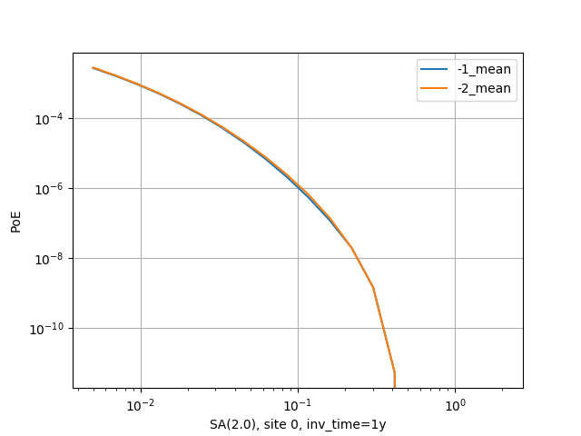
There is a good example of use of the pointsource_distance in the MultiPointClassicalPSHA demo. Here we will just
show a plot displaying the hazard curve without pointsource_distance (with ID=-2) and with pointsource_distance=200 km
(with ID=-1). As you see they are nearly identical but the second calculation is ten times faster.
The pointsource_distance is also crucial when using the point source gridding
approximation: then it can be used to speedup calculations even when the nodal plane and hypocenter distributions are
trivial and no speedup would be expected.
NB: the pointsource_distance approximation has changed a lot across engine releases and you should not expect it to
give always the same results. In particular, in engine 3.8 it has been extended to take into account the fact that small
magnitudes will have a smaller collapse distance. For instance, if you set pointsource_distance=100, the engine will
collapse the ruptures over 100 km for the maximum magnitude, but for lower magnitudes the engine will consider a (much)
shorter collapse distance and will collapse a lot more ruptures. This is possible because given a tectonic region type
the engine knows all the GMPEs associated to that tectonic region and can compute an upper limit for the maximum
intensity generated by a rupture at any distance. Then it can invert the curve and given the magnitude and the maximum
intensity can determine the collapse distance for that magnitude.
In engine 3.11, contrarily to all previous releases, finite side effects are not ignored for distance sites, they are simply averaged over. This gives a better precision. In some case (i.e. the Alaska model) versions of the engine before 3.11 could give a completely wrong hazard on some sites. This is now fixed.
Note: setting pointsource_distance=0 does not completely remove finite size effects. If you want to replace point
sources with points you need to also change the magnitude-scaling relationship to PointMSR. Then the area of the
underlying planar ruptures will be set to 1E-4 squared km and the ruptures will effectively become points.
The linear parameters: width_of_mfd_bin and intensity levels#
The number of ruptures generated by the engine is controlled by the parameter width_of_mfd_bin; for instance if you raise it from 0.1 to 0.2 you will reduce by half the number of ruptures and double the speed of the calculation. It is a linear parameter, at least approximately. Classical calculations are also roughly linear in the number of intensity measure types and levels. A common mistake is to use too many levels. For instance a configuration like the following one:
intensity_measure_types_and_levels = {
  "PGA":  logscale(0.001,4.0, 100),
  "SA(0.3)":  logscale(0.001,4.0, 100),
  "SA(1.0)":  logscale(0.001,4.0, 100)}
requires computing the PoEs on 300 levels. Is that really what the user wants? It could very well be that using only 20 levels per each intensity measure type produces good enough results, while potentially reducing the computation time by a factor of 5.
concurrent_tasks parameter#
There is a last parameter which is worthy of mention, because of its effect on the memory occupation in the risk calculators and in the event based hazard calculator.
- concurrent_tasks:
This is a parameter that you should not set, since in most cases the engine will figure out the correct value to use. However, in some cases, you may be forced to set it. Typically this happens in event based calculations, when computing the ground motion fields. If you run out of memory, increasing this parameter will help, since the engine will produce smaller tasks. Another case when it may help is when computing hazard statistics with lots of sites and realizations, since by increasing this parameter the tasks will contain less sites.
Notice that if the number of concurrent_tasks is too big the performance will get worse and the data transfer will
increase: at a certain point the calculation will run out of memory. I have seen this to happen when generating tens of
thousands of tasks. Again, it is best not to touch this parameter unless you know what you are doing.
Rupture sampling: how to get it wrong#
Rupture samplings is much more complex than one could expect and in many respects surprising. In the many years of existence of the engine, multiple approached were tried and you can expect the details of the rupture sampling mechanism to be different nearly at every version of the engine.
Here we will discuss some tricky points that may help you understand why different versions of the engine may give different results and also why the comparison between the engine and other software performing rupture sampling is nontrivial.
We will start with the first subtlety, the interaction between sampling and filtering. The short version is that you should first sample and then filter.
Here is the long version. Consider the following code emulating rupture sampling for poissonian ruptures:
import numpy

class FakeRupture:
    def __init__(self, mag, rate):
        self.mag = mag
        self.rate = rate

def calc_n_occ(ruptures, eff_time, seed):
    rates = numpy.array([rup.rate for rup in ruptures])
    return numpy.random.default_rng(seed).poisson(rates * eff_time)

mag_rates = [(5.0, 1e-5), (5.1, 2e-5), (5.2, 1e-5), (5.3, 2e-5),
             (5.4, 1e-5), (5.5, 2e-5), (5.6, 1e-5), (5.7, 2e-5)]
fake_ruptures = [FakeRupture(mag, rate) for mag, rate in mag_rates]
eff_time = 50 * 10_000
seed = 42
Running this code will give you the following numbers of occurrence for the 8 ruptures considered:
>> calc_n_occ(fake_ruptures, eff_time, seed)
[ 8  9  6 13  7  6  6 10]
Here we did not consider the fact that engine has a minimum_magnitude feature and it is able to discard ruptures
below the minimum magnitude. But how should it work? The natural approach to follow, for performance-oriented
applications, would be to first discard the low magnitudes and then perform the sampling. However, that would
have effects that would be surprising for most users. Consider the following two alternative:
def calc_n_occ_after_filtering(ruptures, eff_time, seed, min_mag):
    mags = numpy.array([rup.mag for rup in ruptures])
    rates = numpy.array([rup.rate for rup in ruptures])
    return numpy.random.default_rng(seed).poisson(
        rates[mags >= min_mag] * eff_time)

def calc_n_occ_before_filtering(ruptures, eff_time, seed, min_mag):
    mags = numpy.array([rup.mag for rup in ruptures])
    rates = numpy.array([rup.rate for rup in ruptures])
    n_occ = numpy.random.default_rng(seed).poisson(rates * eff_time)
    return n_occ[mags >= min_mag]
Most users would expect that removing a little number of ruptures has a little effect; for instance, if we set
min_mag = 5.1 such that only the first rupture is removed from the total 8 ruptures, we would expect a minor change.
However, if we follow the filter-early approach the user would get completely different occupation numbers:
>> calc_n_occ_after_filtering(fake_ruptures, eff_time, seed, min_mag)
[13  6  9  6 13  7  6]
It is only by using the filter-late approach that the occupation numbers are consistent with the no-filtering case:
>> calc_n_occ_before_filtering(fake_ruptures, eff_time, seed, min_mag)
[ 9  6 13  7  6  6 10]
The problem with the filtering is absolutely general and not restricted only to the magnitude filtering: it is exactly
the same also for distance filtering. Suppose you have a maximum_distance of 300 km and than you decide that you
want to increase it to 301 km. One would expect this change to have a minor impact; instead, you may end up sampling a
very different set of ruptures.
It is true that average quantities like the hazard curves obtained from the ground motion fields will converge for long enough effective time, however in practice you are always in situations were
you cannot perform the calculation for a long enough effective time since it would be computationally prohibitive
you are interested on quantities which are strongly sensitive to aany change, like the Maximum Probable Loss at some return period
In such situations changing the site collection (or changing the maximum distance which is akin to changing the site collection) can change the sampling of the ruptures significantly, at least for engine versions lower than 3.17.
Users wanting to compare the GMFs or the risk on different site collections should be aware of this effect; the solution is to first sample the ruptures without setting any site collection (i.e. disabling the filtering) and then perform the calculation with the site collection starting from the sampled ruptures.