Advanced Calculations#
General#
This manual is for advanced users, i.e. people who already know how to use the engine and have already read the official manual cover-to-cover. If you have just started on your journey of using and working with the OpenQuake engine, this manual is probably NOT for you. Beginners should study the previous sections first. This section is intended for users who are either running large calculations or those who are interested in programatically interacting with the datastore.
For the purposes of this manual a calculation is large if it cannot be run, i.e. if it runs out of memory, it fails with strange errors or it just takes too long to complete.
There are various reasons why a calculation can be too large. 90% of the times it is because the user is making some mistakes and she is trying to run a calculation larger than she really needs. In the remaining 10% of the times the calculation is genuinely large and the solution is to buy a larger machine, or to ask the OpenQuake engine developers to optimize the engine for the specific calculation that is giving issues.
The first things to do when you have a large calculation is to run the command oq info --report job.ini, that will
tell you essential information to estimate the size of the full calculation, in particular the number of hazard sites,
the number of ruptures, the number of assets and the most relevant parameters you are using. If generating the report
is slow, it means that there is something wrong with your calculation and you will never be able to run it completely
unless you reduce it.
The single most important parameter in the report is the number of effective ruptures, i.e. the number of ruptures after distance and magnitude filtering. For instance your report could contain numbers like the following:
#eff_ruptures 239,556
#tot_ruptures 8,454,592
This is an example of a computation which is potentially large - there are over 8 million ruptures generated by the model - but that in practice will be very fast, since 97% of the ruptures will be filtered away. The report gives a conservative estimate, in reality even more ruptures will be discarded.
It is very common to have an unhappy combinations of parameters in the job.ini file, like discretization parameters
that are too small. Then your source model with contain millions and millions of ruptures and the computation will
become impossibly slow or it will run out of memory. By playing with the parameters and producing various reports,
one can get an idea of how much a calculation can be reduced even before running it.
Now, it is a good time to read the section about common mistakes.
Large Calculations in Classical PSHA#
Running large hazard calculations, especially ones with large logic trees, is an art, and there are various techniques that can be used to reduce an impossible calculation to a feasible one.
Reducing a calculation#
The first thing to do when you have a large calculation is to reduce it so that it can run in a reasonable amount of time. For instance you could reduce the number of sites, by considering a small geographic portion of the region interested, of by increasing the grid spacing. Once the calculation has been reduced, you can run it and determine what are the factors dominating the run time.
As we discussed in section about common mistakes, you may want to tweak the quadratic parameters (maximum_distance,
area_source_discretization, rupture_mesh_spacing, complex_fault_mesh_spacing). Also, you may want to choose
different GMPEs, since some are faster than others. You may want to play with the logic tree, to reduce the number of
realizations: this is especially important, in particular for event based calculation were the number of generated
ground motion fields is linear with the number of realizations.
Once you have tuned the reduced computation, you can have an idea of the time required for the full calculation. It will be less than linear with the number of sites, so if you reduced your sites by a factor of 100, the full computation will take a lot less than 100 times the time of the reduced calculation (fortunately). Still, the full calculation can be impossible because of the memory/data transfer requirements, especially in the case of event based calculations. Sometimes it is necessary to reduce your expectations. The examples below will discuss a few concrete cases. But first of all, we must stress an important point:
Our experience tells us that THE PERFORMANCE BOTTLENECKS OF THE
REDUCED CALCULATION ARE TOTALLY DIFFERENT FROM THE BOTTLENECKS OF
THE FULL CALCULATION. Do not trust your performance intuition.
Collapsing the GMPE logic tree#
Some hazard models have GMPE logic trees which are insanely large. For instance the GMPE logic tree for the latest European model (ESHM20) contains 961,875 realizations. This causes two issues:
it is impossible to run a calculation with full enumeration, so one must use sampling
when one tries to increase the number of samples to study the stability of the mean hazard curves, the calculation runs out of memory
Fortunately, it is possible to compute the exact mean hazard curves by collapsing the GMPE logic tree. This is a simple as listing the name of the branchsets in the GMPE logic tree that one wants to collapse. For instance in the case of ESHM20 model there are the following 6 branchsets:
Shallow_Def (19 branches)
CratonModel (15 branches)
BCHydroSubIF (15 branches)
BCHydroSubIS (15 branches)
BCHydroSubVrancea (15 branches)
Volcanic (1 branch)
By setting in the job.ini the following parameters:
number_of_logic_tree_samples = 0
collapse_gsim_logic_tree = Shallow_Def CratonModel BCHydroSubIF BCHydroSubIS BCHydroSubVrancea Volcanic
it is possible to collapse completely the GMPE logic tree, i.e. going from 961,875 realizations to 1. Then the memory issues are solved and one can assess the correct values of the mean hazard curves. Then it is possible to compare with the value produce with sampling and assess how much they can be trusted.
NB: the collapse_gsim_logic_tree feature is rather old but only for engine versions >=3.13 it produces the exact
mean curves (using the AvgPoeGMPE); otherwise it will produce a different kind of collapsing (using the AvgGMPE).
disagg_by_src#
Given a system of various sources affecting a specific site, one very common question to ask is: what are the more
relevant sources, i.e. which sources contribute the most to the mean hazard curve? The engine is able to answer such
question by setting the disagg_by_src flag in the job.ini file. When doing that, the engine saves in the datastore a
4-dimensional ArrayWrapper called mean_rates_by_src with dimensions (site ID, intensity measure type, intensity measure
level, source ID). From that it is possible to extract the contribution of each source to the mean hazard curve
(interested people should look at the code in the function check_disagg_by_src). The ArrayWrapper mean_rates_by_src
can also be converted into a pandas DataFrame, then getting something like the following:
>> dstore['mean_rates_by_src'].to_dframe().set_index('src_id')
               site_id  imt  lvl         value
ASCTRAS407           0  PGA    0  9.703749e-02
IF-CFS-GRID03        0  PGA    0  3.720510e-02
ASCTRAS407           0  PGA    1  6.735009e-02
IF-CFS-GRID03        0  PGA    1  2.851081e-02
ASCTRAS407           0  PGA    2  4.546237e-02
...                ...  ...  ...           ...
IF-CFS-GRID03        0  PGA   17  6.830692e-05
ASCTRAS407           0  PGA   18  1.072884e-06
IF-CFS-GRID03        0  PGA   18  1.275539e-05
ASCTRAS407           0  PGA   19  1.192093e-07
IF-CFS-GRID03        0  PGA   19  5.960464e-07
The value field here is the probability of exceedence in the hazard curve. The lvl field is an integer
corresponding to the intensity measure level in the hazard curve.
In engine 3.15 we introduced the so-called “colon convention” on source IDs: if you have many sources that for some
reason should be collected together - for instance because they all account for seismicity in the same tectonic region,
or because they are components of a same source but are split into separate sources by magnitude - you can tell the
engine to collect them into one source in the mean_rates_by_src matrix. The trick is to use IDs with the same
prefix, a colon, and then a numeric index. For instance, if you had 3 sources with IDs src_mag_6.65, src_mag_6.75,
src_mag_6.85, fragments of the same source with different magnitudes, you could change their IDs to something like
src:0, src:1, src:2 and that would reduce the size of the matrix mean_rates_by_src by 3 times by collecting
together the contributions of each source. There is no restriction on the numeric indices to start from 0, so using the
names src:665, src:675, src:685 would work too and would be clearer: the IDs should be unique, however.
If the IDs are not unique and the engine determines that the underlying sources are different, then an extension
“semicolon + incremental index” is automatically added. This is useful when the hazard modeler wants to define a model
where the more than one version of the same source appears in one source model, having changed some of the parameters,
or when varied versions of a source appear in each branch of a logic tree. In that case, the modeler should use always
the exact same ID (i.e. without the colon and numeric index): the engine will automatically distinguish the sources
during the calculation of the hazard curves and consider them the same when saving the array mean_rates_by_src: you
can see an example in the test qa_tests_data/classical/case_20/job_bis.ini in the engine code base. In that case
the source_info dataset will list 7 sources CHAR1;0 CHAR1;1 CHAR1;2 COMFLT1;0 COMFLT1;1 SFLT1;0 SFLT1;1 but the
matrix mean_rates_by_src will see only three sources CHAR1 COMFLT1 SFLT1 obtained by composing together the
versions of the underlying sources.
In version 3.15 mean_rates_by_src was extended to work with mutually exclusive sources, i.e. for the Japan model.
You can see an example in the test qa_tests_data/classical/case_27. However, the case of mutually exclusive ruptures
- an example is the New Madrid cluster in the USA model - is not supported yet.
In some cases it is tricky to discern whether use of the colon convention or identical source IDs is appropriate. The following list indicates several possible cases that a user may encounter, and the appropriate approach to assigning source IDs. Note that this list includes the cases that have been tested so far, and is not a comprehensive list of all cases that may arise.
Sources in the same source group/source model are scaled alternatives of each other. For example, this occurs when for a given source, epistemic uncertainties such as occurrence rates or geometries are considered, but the modeller has pre-scaled the rates rather than including the alternative hypothesis in separate logic tree branches.
Naming approach: identical IDs.
Sources in different files are alternatives of each other, e.g. each is used in a different branch of the source model logic tree.
Naming approach: identical IDs.
A source is defined in OQ by numerous sources, either in the same file or different ones. For example, one could have a set of non-parametric sources, each with many ruptures, that are grouped together into single files by magnitude. Or, one could have many point sources that together represent the seismicity from one source.
Naming approach: colon convention
One source consists of many mutually exclusive sources, as in qa_tests_data/classical/case_27.
Naming approach: colon convention
Cases 1 and 2 could include include more than one source typology, as in qa_tests_data/classical/case_79.
NB: disagg_by_src can be set to true only if the ps_grid_spacing approximation is disabled. The reason is that
the ps_grid_spacing approximation builds effective sources which are not in the original source model, thus breaking
the connection between the values of the matrix and the original sources.
The post-processing framework and Vector-valued PSHA calculations#
Since version 3.17 the OpenQuake engine has special support for custom postprocessors. A postprocessor is a Python
module located in the directory openquake/calculators/postproc and containing a main function with signature:
def main(dstore, [csm], ...):
    ...
Post-processors are called after a classical or preclassical calculation: the dstore parameter is a DataStore
instance corresponding to the calculation, while the csm parameter is a CompositeSourceModel instance (it can be
omitted if not needed).
The main function is called when the user sets in the job.ini file the parameters postproc_func and postproc_args.
postproc_func is the dotted name of the postprocessing function (in the form modulename.funcname where funcname
is normally main) and postproc_args is a dictionary of literal arguments that get passed to the function; if not
specified the empty dictionary is passed. This happens for instance for the conditional spectrum post-processor since it
does not require additional arguments with respect to the ones in dstore['oqparam'].
The post-processing framework was put in place in order to run VPSHA calculations. The user can find an example in
qa_tests_data/postproc/case_mrd. In the job.ini file there are the lines:
postproc_func = compute_mrd.main
postproc_args = {
  'imt1': 'PGA',
  'imt2': 'SA(0.05)',
  'cross_correlation': 'BakerJayaram2008',
  'seed': 42,
  'meabins': [0.1, 0.2, 0.3, 0.4, 0.5, 0.6],
  'sigbins': [0.2, 0.3, 0.4, 0.5, 0.6, 0.7],
  'method': 'indirect'}
while the postprocessor module openquake.calculators.postproc.compute_mrd contains the function:
# inside openquake.calculators.postproc.compute_mrd
def main(dstore, imt1, imt2, cross_correlation, seed, meabins, sigbins,
         method='indirect'):
    ...
Inside main there is code to create the dataset mrd which contains the Mean Rate Distribution as an array of
shape L1 x L1 x N where L1 is the number of levels per IMT minus 1 and N the number of sites (normally 1).
While the postprocessing part for VPSHA calculations is computationally intensive, it is much more common to have a
light postprocessing, i.e. faster than the classical calculation it depends on. In such situations the postprocessing
framework really shines, since it is possible to reuse the original calculation via the standard --hc switch, i.e. you
can avoid repeating multiple times the same classical calculation if you are interested in running the postprocessor
with different parameters. In that situation the main function will get a DataStore instance with an attribute parent
corresponding to the DataStore of the original calculation.
The postprocessing framework also integrates very well with interactive development (think of Jupyter notebooks). The following lines are all you need to create a child datastore where the postprocessing function can store its results after reading the data from the calculation datastore:
>> from openquake.commonlib.datastore import read, build_dstore_log
>> from openquake.calculators.postproc import mypostproc
>> dstore, log = build_dstore_log(parent=read(calc_id))
>> with log:
..     mypostproc.main(dstore)
The conditional spectrum post-processor#
Since version 3.17 the engine includes an experimental post-processor which is able to compute the conditional spectrum.
The implementation was adapted from the paper Conditional Spectrum Computation Incorporating Multiple Causal Earthquakes and Ground-Motion Prediction Models by Ting Lin, Stephen C. Harmsen, Jack W. Baker, and Nicolas Luco (http://citeseerx.ist.psu.edu/viewdoc/download?doi=10.1.1.845.163&rep=rep1&type=pdf) and it is rather sophisticated.
In order to perform a conditional spectrum calculation you need to specify, in addition to the usual parameter of a classical calculation:
a reference intensity measure type (i.e. imt_ref = SA(0.2))
a cross correlation model (i.e. cross_correlation = BakerJayaram2008)
a set of poes (i.e. poes = 0.01 0.1)
The engine will compute a mean conditional spectrum for each poe and site, as well as the usual mean uniform hazard
spectra. The following restrictions are enforced:
the IMTs can only be of type
SAandPGAthe source model cannot contain mutually exclusive sources (i.e. you cannot compute the conditional spectrum for the Japan model)
An example can be found in the engine repository, in the directory openquake/qa_tests_data/conditional_spectrum/case_1. If you run it, you will get something like the following:
$ oq engine --run job.ini
...
 id | name
261 | Full Report
262 | Hazard Curves
260 | Mean Conditional Spectra
263 | Realizations
264 | Uniform Hazard Spectra
Exporting the output 260 will produce two files conditional-spectrum-0.csv and conditional-spectrum-1.csv; the
first will refer to the first poe, the second to the second poe. Each file will have a structure like the following:
 #,,,,"generated_by='OpenQuake engine 3.13.0-gitd78d717e66', start_date='2021-10-13T06:15:20', checksum=3067457643, imls=[0.99999, 0.61470], site_id=0, lon=0.0, lat=0.0"
sa_period,val0,std0,val1,std1
0.00000E+00,1.02252E+00,2.73570E-01,7.53388E-01,2.71038E-01
1.00000E-01,1.99455E+00,3.94498E-01,1.50339E+00,3.91337E-01
2.00000E-01,2.71828E+00,9.37914E-09,1.84910E+00,9.28588E-09
3.00000E-01,1.76504E+00,3.31646E-01,1.21929E+00,3.28540E-01
1.00000E+00,3.08985E-01,5.89767E-01,2.36533E-01,5.86448E-01
The number of columns will depend from the number of sites. The conditional spectrum calculator, like the disaggregation
calculator, is meant to be run on a very small number of sites, normally one. In this example there are two sites 0 and 1
and the columns val0 and val give the value of the conditional spectrum on such sites respectively, while the
columns std0 and std1 give the corresponding standard deviations.
Conditional spectra for individual realizations are also computed and stored for debugging purposes, but they are not exportable.
Event Based and Scenarios#
Scenario risk calculations usually do not pose a performance problem, since they involve a single rupture and limited geographical region for analysis. Some event-based risk calculations, however, may involve millions of ruptures and exposures spanning entire countries or even continents. This section offers some practical tips for running large event-based risk calculations, especially ones involving large logic trees, and proposes techniques that might be used to make an otherwise intractable calculation tractable.
Understanding the hazard#
Event-based calculations are typically dominated by the hazard component (unless there are lots of assets aggregated on a few hazard sites) and therefore the first thing to do is to estimate the size of the hazard, i.e. the number of GMFs that will be produced. Since we are talking about a large calculation, first of all, we need to reduce it to a size that is guaranteed to run quickly. The simplest way to do that is to reduce the parameters directly affecting the number of ruptures generated, i.e.
investigation_time
ses_per_logic_tree_path
number_of_logic_tree_samples
For instance, if you have ses_per_logic_tree_path = 10,000 reduce it to 10, run the calculation and you will see in
the log something like this:
[2018-12-16 09:09:57,689 #35263 INFO] Received
{'gmfdata': '752.18 MB', 'hcurves': '224 B', 'indices': '29.42 MB'}
The amount of GMFs generated for the reduced calculation is 752.18 MB; and since the calculation has been reduced by a factor of 1,000, the full computation is likely to generate around 750 GB of GMFs. Even if you have sufficient disk space to store this large quantity of GMFs, most likely you will run out of memory. Even if the hazard part of the calculation manages to run to completion, the risk part of the calculation is very likely to fail — managing 750 GB of GMFs is beyond the current capabilities of the engine. Thus, you will have to find ways to reduce the size of the computation.
A good start would be to carefully set the parameters minimum_magnitude and minimum_intensity:
minimum_magnitudeis a scalar or a dictionary keyed by tectonic region; the engine will discard ruptures with magnitudes below the given thresholdsminimum_intensityis a scalar or a dictionary keyed by the intensity measure type; the engine will discard GMFs below the given intensity thresholds
Choosing reasonable cutoff thresholds with these parameters can significantly reduce the size of your computation when there are a large number of small magnitude ruptures or low intensity GMFs being generated, which may have a negligible impact on the damage or losses, and thus could be safely discarded.
region_grid_spacing#
In our experience, the most common error made by our users is to compute the hazard at the sites of the exposure. The issue is that it is possible to have exposures with millions of assets on millions of distinct hazard sites. Computing the GMFs for millions of sites is hard or even impossible (there is a limit of 4 billion rows on the size of the GMF table in the datastore). Even in the cases when computing the hazard is possible, then computing the risk starting from an extremely large amount of GMFs will likely be impossible, due to memory/runtime constraints.
The second most common error is using an extremely fine grid for the site model. Remember that if you have a resolution of 250 meters, a square of 250 km x 250 km will contain one million sites, which is definitely too much. The engine was designed when the site models had resolutions around 5-10 km, i.e. of the same order of the hazard grid, while nowadays the vs30 fields have a much larger resolution.
Both problems can be solved in a simple way by specifying the region_grid_spacing parameter. Make it large enough
that the resulting number of sites becomes reasonable and you are done. You will lose some precision, but that is
preferable to not being able to run the calculation. You will need to run a sensitivity analysis with different values
of region_grid_spacing parameter to make sure that you get consistent results, but that’s it.
Once a region_grid_spacing is specified, the engine computes the convex hull of the exposure sites and builds a
grid of hazard sites, associating the site parameters from the closest site in the site model and discarding sites in
the region where there are no assets (i.e. more distant than region_grid_spacing * sqrt(2)). The precise logic is
encoded in the function openquake.commonlib.readinput.get_sitecol_assetcol, if you want to know the specific
implementation details.
Our recommendation is to use the command oq prepare_site_model to apply such logic before starting a calculation and
thus producing a custom site model file tailored to your exposure (see the section prepare_site_model).
Collapsing of branches#
When one is not interested in the uncertainty around the loss estimates and cares more about the mean estimates, all of the source model branches can be “collapsed” into one branch. Using the collapsed source model should yield the same mean hazard or loss estimates as using the full source model logic tree and then computing the weighted mean of the individual branch results.
Similarly, the GMPE logic tree for each tectonic region can also be “collapsed” into a single branch. Using a single collapsed GMPE for each TRT should also yield the same mean hazard estimates as using the full GMPE logic tree and then computing the weighted mean of the individual branch results. This has become possible through the introduction of AvgGMPE feature in version 3.9.
Splitting the calculation into subregions#
If one is interested in propagating the full uncertainty in the source models or ground motion models to the hazard or loss estimates, collapsing the logic trees into a single branch to reduce computational expense is not an option. But before going through the effort of trimming the logic trees, there is an interim step that must be explored, at least for large regions, like the entire continental United States. This step is to geographically divide the large region into logical smaller subregions, such that the contribution to the hazard or losses in one subregion from the other subregions is negligibly small or even zero. The effective realizations in each of the subregions will then be much fewer than when trying to cover the entire large region in a single calculation.
Trimming of the logic-trees or sampling of the branches#
Trimming or sampling may be necessary if the following two conditions hold:
You are interested in propagating the full uncertainty to the hazard and loss estimates; only the mean or quantile results are not sufficient for your analysis requirements, AND
The region of interest cannot be logically divided further as described above; the logic-tree for your chosen region of interest still leads to a very large number of effective realizations.
Sampling is the easier of the two options now. You only need to ensure that you sample a sufficient number of branches to capture the underlying distribution of the hazard or loss results you are interested in. The drawback of random sampling is that you may still need to sample hundreds of branches to capture well the underlying distribution of the results.
Trimming can be much more efficient than sampling, because you pick a few branches such that the distribution of the hazard or loss results obtained from a full-enumeration of these branches is nearly the same as the distribution of the hazard or loss results obtained from a full-enumeration of the entire logic-tree.
Extra tips specific to event based calculations#
Event based calculations differ from classical calculations because they produce visible ruptures, which can be
exported and made accessible to the user. In classical calculations, instead, the underlying ruptures only live in
memory and are normally not saved in the datastore, nor are exportable. The limitation is fundamentally a technical one:
in the case of an event based calculation only a small fraction of the ruptures contained in a source are actually
generated, so it is possible to store them. In a classical calculation all ruptures are generated and there are so many
millions of them that it is impractical to save them, unless there are very few sites. For this reason they live in
memory, they are used to produce the hazard curves and immediately discarded right after. The exception if for the case
of few sites, i.e. if the number of sites is less than the parameter max_sites_disagg which by default is 10.
Convergency of the GMFs for non-trivial logic trees#
In theory, the hazard curves produced by an event based calculation should converge to the curves produced by an
equivalent classical calculation. In practice, if the parameters number_of_logic_tree_samples and
ses_per_logic_tree_path (the product of them is the relevant one) are not large enough they may be different. The
engine is able to compare the mean hazard curves and to see how well they converge. This is done automatically if the
option mean_hazard_curves = true is set. Here is an example of how to generate and plot the curves for one of our
QA tests (a case with bad convergence was chosen on purpose):
$ oq engine --run event_based/case_7/job.ini
<snip>
WARNING:root:Relative difference with the classical mean curves for IMT=SA(0.1): 51%
WARNING:root:Relative difference with the classical mean curves for IMT=PGA: 49%
<snip>
$ oq plot /tmp/cl/hazard.pik /tmp/hazard.pik --sites=0,1,2
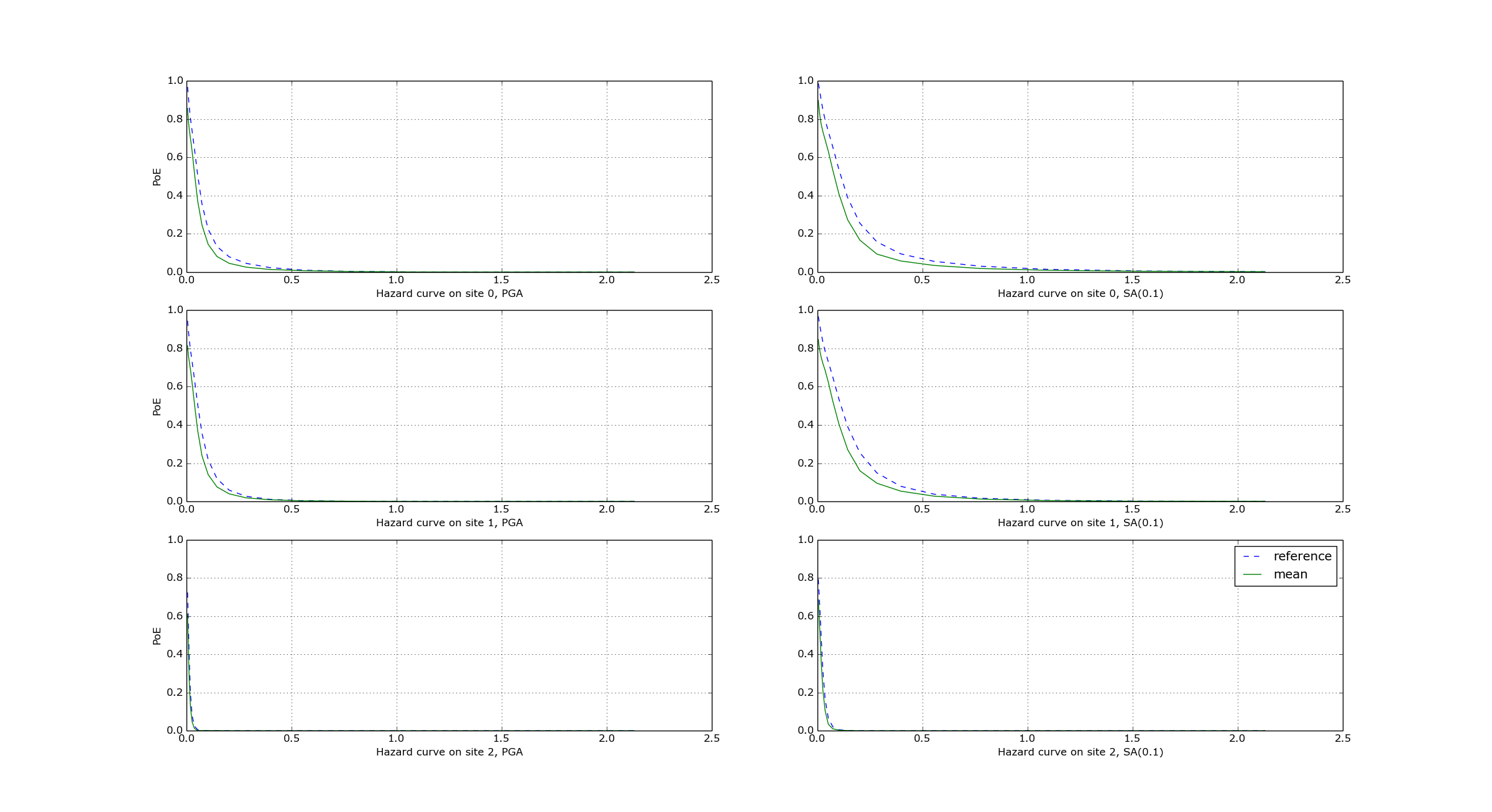
The relative difference between the classical and event based curves is computed by computing the relative difference between each point of the curves for each curve, and by taking the maximum, at least for probabilities of exceedence larger than 1% (for low values of the probability the convergency may be bad). For the details I suggest you to look at the code.
Risk profiles#
The OpenQuake engine can produce risk profiles, i.e. estimates of average losses and maximum probable losses for all countries in the world. Even if you are interested in a single country, you can still use this feature to compute risk profiles for each province in your country.
However, the calculation of the risk profiles is tricky and there are actually several different ways to do it.
The least-recommended way is to run independent calculations, one for each country. The issue with this approach is that even if the hazard model is the same for all the countries (say you are interested in the 13 countries of South America), due to the nature of event based calculations, different ruptures will be sampled in different countries. In practice, when comparing Chile with Peru you will see differences due to the fact that the random sampling picked different ruptures in the two contries and not real differences. In theory, the effect should disappear if the calculations have sufficiently long investigation times, when all possible ruptures are sampled, but in practice, for finite investigation times there will always be different ruptures.
To avoid such issues, the country-specific calculations should ideally all start from the same set of precomputed ruptures. You can compute the whole stochastic event set by running an event based calculation without specifying the sites and with the parameter
ground_motion_fieldsset to false. Currently, one must specify a few global site parameters in the precalculation to make the engine checker happy, but they will not be used since the ground motion fields will not be generated in the precalculation. The ground motion fields will be generated on-the-fly in the subsequent individual country calculations, but not stored in the file system. This approach is fine if you do not have a lot of disk space at your disposal, but it is still inefficient since it is quite prone to the slow tasks issue.If you have plenty of disk space it is better to also generate the ground motion fields in the precalculation, and then run the contry-specific risk calculations starting from there. This is particularly convenient if you foresee the need to run the risk part of the calculations multiple times, while the hazard part remains unchanged. Using a precomputed set of GMFs removes the need to rerun the hazard part of the calculations each time. This workflow has been particularly optimized since version 3.16 of the engine and it is now quite efficient.
If you have a really powerful machine, the simplest is to run a single calculation considering all countries in a single job.ini file. The risk profiles can be obtained by using the
aggregate_byandreaggregate_byparameters. This approach can be much faster than the previous ones. However, approaches #2 and #3 are cloud-friendly and can be preferred if you have access to cloud-computing resources, since then you can spawn a different machine for each country and parallelize horizontally.
Here are some tips on how to prepare the required job.ini files:
When using approach #1 you will have 13 different files (in the example of South America) with a format like the following:
$ cat job_Argentina.ini
calculation_mode = event_based_risk
source_model_logic_tree_file = ssmLT.xml
gsim_logic_tree_file = gmmLTrisk.xml
site_model_file = Site_model_Argentina.csv
exposure_file = Exposure_Argentina.xml
...
$ cat job_Bolivia.ini
calculation_mode = event_based_risk
source_model_logic_tree_file = ssmLT.xml
gsim_logic_tree_file = gmmLTrisk.xml
site_model_file = Site_model_Bolivia.csv
exposure_file = Exposure_Bolivia.xml
...
Notice that the source_model_logic_tree_file and gsim_logic_tree_file
will be the same for all countries since the hazard model is the same;
the same sources will be read 13 times and the ruptures will be sampled
and filtered 13 times. This is inefficient. Also, hazard parameters like
truncation_level = 3
investigation_time = 1
number_of_logic_tree_samples = 1000
ses_per_logic_tree_path = 100
maximum_distance = 300
must be the same in all 13 files to ensure the consistency of the calculation. Ensuring this consistency can be prone to human error.
When using approach #2 you will have 14 different files: 13 files for the individual countries and a special file for precomputing the ruptures:
$ cat job_rup.ini
calculation_mode = event_based
source_model_logic_tree_file = ssmLT.xml
gsim_logic_tree_file = gmmLTrisk.xml
reference_vs30_value = 760
reference_depth_to_1pt0km_per_sec = 440
ground_motion_fields = false
...
The files for the individual countries will be as before, except for
the parameter source_model_logic_tree_file which should be
removed. That will avoid reading 13 times the same source model files,
which are useless anyway, since the calculation now starts from
precomputed ruptures. There are still a lot of repetitions in the
files and the potential for making mistakes.
Approach #3 is very similar to approach #2: the only differences will be
in the initial file, the one used to precompute the GMFs. Obviously it
will require setting ground_motion_fields = true; moreover, it will
require specifying the full site model as follows:
site_model_file =
  Site_model_Argentina.csv
  Site_model_Bolivia.csv
  ...
The engine will automatically concatenate the site model files for all
13 countries and produce a single site collection. The site parameters
will be extracted from such files, so the dummy global parameters
reference_vs30_value, reference_depth_to_1pt0km_per_sec, etc
can be removed.
It is FUNDAMENTAL FOR PERFORMANCE to have reasonable site model files, i.e. you should not compute the hazard at the location of every single asset, but rather you should use a variable-size grid fitting the exposure.
The engine provides a command oq prepare_site_model
which is meant to generate sensible site model files starting from
the country exposures and the global USGS vs30 grid.
It works by using a hazard grid so that the number of sites
can be reduced to a manageable number. Please refer to the manual in
the section about the oq commands to see how to use it, or try
oq prepare_site_model --help.
For reference, we were able to compute the hazard for all of South America on a grid of half million sites and 1 million years of effective time in a few hours in a machine with 120 cores, generating half terabyte of GMFs. The difficult part is avoiding running out memory when running the risk calculation; huge progress in this direction was made in version 3.16 of the engine.
Approach #4 is the best, when applicable, since there is only a single file,
thus avoiding entirely the possibily of having inconsistent parameters
in different files. It is also the faster approach, not to mention the
most convenient one, since you have to manage a single calculation and
not 13. That makes the task of managing any kind of post-processing a lot
simpler. Unfortunately, it is also the option that requires more
memory and it can be infeasable if the model is too large and you do not
have enough computing resources. In that case your best bet might be to
go back to options #2 or #3. If you have access to multiple small machines,
approaches #2 and #3 can be more attractive than #4, since then you
can scale horizontally. If you decide to use approach #4,
in the single file you must specify the site_model_file as done in
approach #3, and also the exposure_file as follows:
exposure_file =
  Exposure_Argentina.xml
  Exposure_Bolivia.xml
  ...
The engine will automatically build a single asset collection for the
entire continent of South America. In order to use this approach, you
need to collect all the vulnerability functions in a single file and
the taxonomy mapping file must cover the entire exposure for all
countries. Moreover, the exposure must contain the associations
between asset<->country; in GEM’s exposure models, this is typically
encoded in a field called ID_0. Then the aggregation by country
can be done with the option
aggregate_by = ID_0
Sometimes, one is interested in finer aggregations, for instance by country and also by occupancy (Residential, Industrial or Commercial); then you have to set
aggregate_by = ID_0, OCCUPANCY
reaggregate_by = ID_0
reaggregate_by` is a new feature of engine 3.13 which allows to go
from a finer aggregation (i.e. one with more tags, in this example 2)
to a coarser aggregation (i.e. one with fewer tags, in this example 1).
Actually the command ``oq reaggregate
has been there for more than one
year; the new feature is that it is automatically called at the end of
a calculation, by spawning a subcalculation to compute the reaggregation.
Without reaggregate_by the aggregation by country would be lost,
since only the result of the finer aggregation would be stored.
Single-line commands#
When using approach #1 your can run all of the required calculations with the command:
$ oq engine --run job_Argentina.csv job_Bolivia.csv ...
When using approach #2 your can run all of the required calculations with the command:
$ oq engine --run job_rup.ini job_Argentina.csv job_Bolivia.csv ...
When using approach #3 your can run all of the required calculations with the command:
$ oq engine --run job_gmf.ini job_Argentina.csv job_Bolivia.csv ...
When using approach #4 your can run all of the required calculations with the command:
$ oq engine --run job_all.ini
Here job_XXX.ini are the country specific configuration files,
job_rup.ini is the file generating the ruptures, job_rup.ini
is the file generating the ruptures, job_gmf.ini is the file
generating the ground motion files and job_all.ini is the
file encompassing all countries.
Finally, if you have a file job_haz.ini generating the full GMFs,
a file job_weak.ini generating the losses with a weak building code
and a file job_strong.ini generating the losses with a strong building
code, you can run the entire an analysis with a single command as follows:
$ oq engine --run job_haz.ini job_weak.ini job_strong.ini
This will generate three calculations and the GMFs will be reused. This is as efficient as possible for this kind of problem.
Caveat: GMFs are split-dependent#
You should not expect the results of approach #4 to match exactly the results of approaches #3 or #2, since splitting a calculation by countries is a tricky operation. In general, if you have a set of sites and you split it in disjoint subsets, and then you compute the ground motion fields for each subset, you will get different results than if you do not split.
To be concrete, if you run a calculation for Chile and then one for Argentina, you will get different results than running a single calculation for Chile+Argentina, even if you have precomputed the ruptures for both countries, even if the random seeds are the same and even if there is no spatial correlation. Many users are surprised but this fact, but it is obvious if you know how the GMFs are computed. Suppose you are considering 3 sites in Chile and 2 sites in Argentina, and that the value of the random seed in 123456: if you split, assuming there is a single event, you will produce the following 3+2 normally distributed random numbers:
>>> np.random.default_rng(123456).normal(size=3)  # for Chile
array([ 0.1928212 , -0.06550702,  0.43550665])
>>> np.random.default_rng(123456).normal(size=2)  # for Argentina
array([ 0.1928212 , -0.06550702])
If you do not split, you will generate the following 5 random numbers instead:
>>> np.random.default_rng(123456).normal(size=5)
array([ 0.1928212 , -0.06550702,  0.43550665,  0.88235875,  0.37132785])
They are unavoidably different. You may argue that not splitting is the correct way of proceeding, since the splitting causes some random numbers to be repeated (the numbers 0.1928212 and -0.0655070 in this example) and actually breaks the normal distribution.
In practice, if there is a sufficiently large event-set and if you are interested in statistical quantities, things work out and you should see similar results with and without splitting. But you will never produce identical results. Only the classical calculator does not depend on the splitting of the sites, for event based and scenario calculations there is no way out.