Physical Risk Input Description#
The main sources of input information required for a risk calculation with the OpenQuake engine are an exposure model and a physical vulnerability model or fragility model (in addition to the calculation type and the region of interest). An exposure model for a given category of asset (e.g. population, buildings, contents) describes, at each location of interest within a given region, the value of each asset of a given taxonomy. The physical vulnerability model described the loss ratio distribution for a set of intensity measure levels, while the fragility model provides the probability of exceeding a set of damage states, given a set of intensity measure levels.
Exposure#
The OpenQuake engine requires an exposure model that needs to be stored according to the respective Natural hazards’ Risk Markup Language (NRML) schema (see oq-nrmllib). More information on the formats of this input model is provided in the OpenQuake Engine User Manual. This file format can include several typologies of asset such as population or buildings. The following parameters are currently being used to describe each asset in the exposure model:
Asset reference: A unique key used to identify the asset instance;
Location: Geographic coordinates of the asset expressed in decimal degrees;
Taxonomy: Reference to the classification scheme that describes the asset;
Number: A numerical value describing the number of units at the given location (e.g. building count).
Area: This parameter specifies the built-up area of the asset, and can be defined in the two following ways: the aggregated area (i.e. the total built-up area of all the units at a given location, with a certain taxonomy); area per unit (i.e. the average built-up area for a single building);
Structural cost: This parameter represents the structural replacement cost of the asset. This value can be defined in three possible ways: the aggregated structural cost (i.e. the total economic value of all the units with a certain taxonomy at a given location); the cost per unit (i.e. the average value for a single building); the cost per unit of area. Further information about how the structural cost is handled within the OpenQuake engine can be found in the OpenQuake Engine User Manual.
Non-structural cost: This parameter is used to define the cost of the non-structural components. This cost defined in the same way as the structural cost.
Contents cost: This parameter is used to define the contents cost, and it can be defined in the same way as the structural cost.
Retrofitting cost: This parameter is used to define the economic structural cost due to the implementation of a retrofitting/strengthening intervention. The retrofitting cost can be defined in the same way as the structural cost.
Occupants: This parameter defines the number of people that might exist inside of a given structure. Different values of occupants can be stored according to the time of the day (e.g day, night, transit).
Deductible: This parameter is used in the computation of the insured losses, and it establishes the economic value that needs to be deducted from the ground-up losses. A deductible needs to be defined for each cost type (structural, non-structural and contents). This threshold can be defined in two ways:
the direct (absolute) value that will be deducted;
the fraction (relative) of the total cost that will be deducted.
Limit: This parameter establishes the maximum economic amount that can be insured, and it also needs to be defined for each cost type. The limit can also be defined as an absolute or relative quantity.
Physical Vulnerability#
Physical vulnerability is defined as the probabilistic distribution of loss, given an intensity measure level. These vulnerability functions can be derived directly, usually through empirical methods where the losses from past events at given locations are related to the levels of intensity of ground motion at those locations, or they can be derived by combining fragility functions and consequence functions. Fragility functions describe the probability of exceeding a set of limit states, given an intensity measure level; limit states describe the limits to performance levels, such as damage or injury levels. Fragility functions can be derived by expert-opinion, empirically (using observed data), or analytically, by explicitly modeling the behavior of a given asset typology when subjected to increasing levels of ground motion. Consequence functions describe the probability distribution of loss, given a performance level and are generally derived empirically.
Version 1.0 of the OpenQuake engine only supports physical vulnerability through the aforementioned vulnerability functions. As part of the plans for a risk modelling toolkit, calculators are envisaged that will combine fragility functions and consequence functions to produce vulnerability functions that can be input into the engine.
Vulnerability Functions#
Discrete Vulnerability Functions#
In the current version of the OpenQuake engine (v1.0) discrete vulnerability functions are used to directly estimate fatalities and economic losses due to physical damage. Discrete vulnerability functions are described by a list of intensity measure levels and corresponding mean loss ratios (the ratio of mean loss to exposed value), associated coefficients of variation and probability distributions. The uncertainty on the loss ratio can follow a lognormal or Beta distribution. The figure below illustrates a discrete vulnerability function.
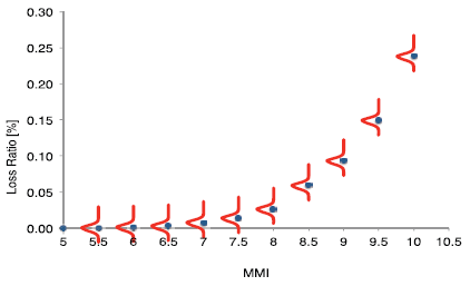
Discrete vulnerability function.#
Continuous Vulnerability Functions#
Continuous vulnerability functions may be implemented in future versions of the OpenQuake Continuous engine. Continuous vulnerability functions will probably be described by continuous distribu- tions of mean loss ratio and other fractiles of loss ratio, with ground motion intensity. The figure below illustrates this type of function, showing the distribution of mean loss and the 10 percent and 90 percent fractiles.
Fragility Functions#
Fragility functions describe the probability of exceeding a set of limit states, given an intensity measure level. When the asset category concerns structures (e.g. buildings), the intensity measure can either be structure-independent or structure-dependent. The former can be calculated directly from recorded measurements of ground shaking (e.g. peak ground accel- eration, peak ground velocity, spectral acceleration at a given period of vibration, or even macroseismic intensity). The latter requires information on the characteristics of the struc- tures in order to be calculated, for example spectral acceleration at the fundamental period of vibration, or spectral displacement at the limit state period of vibration. The calculation of these structural characteristics might be through a simple formulae (e.g. a yield period- height equation, see e.g. Crowley and Pinho [2004]) or through so-called non-linear static methods, which are needed when the intensity measure is a non-linear response quantity such as spectral displacement at the limit state period of vibration (see e.g. FEMA-440:ATC [2005]). The oq-risklib currently does not support non-linear static methods.
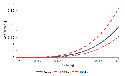
Continuous vulnerability function.#
Discrete Fragility Functions#
Fragility functions can be defined in a discrete way by providing, for each limit state, a list of intensity measure levels and respective probabilities of exceedance. The first figure below presents a set of discrete fragility functions using a macroseismic intensity measure.
Continuous Fragility Functions#
Continuous fragility functions are defined by the parameters of a cumulative distribution function. In the second figure below an example of a set of continuous fragility functions with a structure- dependent intensity measure is presented.
Uncertainty in Fragility Functions#
The uncertainty in continuous fragility functions will be accounted for in future versions of the engine. The third figure below shows a lognormal distribution that has been fit to the data (i.e. the fragility function), and the probabilistic distribution (i.e. mean and standard deviation) to describe the uncertainty in both the logarithmic mean and logarithmic standard deviation of the fragility function. When a set of fragility functions for different limit states are used, it is also necessary to provide information on the correlation between the logarithmic means and logarithmic standard deviations of each limit state.
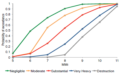
Set of discrete fragility functions.#
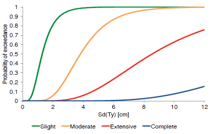
Set of continuous fragility functions.#
Consequence Functions#
Consequence functions describe the probability distribution of loss, given a performance level. For example, if the asset category is buildings and the performance level is significant damage, the consequence function will describe the mean loss ratio, coefficient of variation and probability distribution for that level of damage. The second figure below presents the mean damage ratios for a set of performance levels proposed by two different sources. Although these functions are not directly supported, users can combine consequence functions with fragility functions to produce vulnerability functions to be input into the engine.
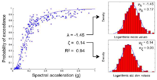
Uncertainty of continuous fragility functions.#

Consequence functions adapted from Bal et al. [2010]#