Calculation Examples#
This chapter presents some hazard results computed with the OpenQuake engine. By considering simple synthetic test cases, we illustrate the behaviour of a number of algorithms underlying the seismic source modelling and the logic tree processing. We also present examples of PSHA performed using the 2008 U.S. national seismic hazard model (Petersen et al., 2008) to illustrate the capabilities of the OpenQuake engine when dealing with complex models.
Classical PSHA with an Area Source#
We consider here the case of a single area source. The source has a circular shape and a radious of 200 km. The activity is described by a truncated Gutenberg-Richter magnitude frequency distribution, with minimum magnitude equal to 5 and maximum magnitude equal to 6.5. The a-value is 5 and b-value is 1. The seismogenic layer extends from 0 to 20 km. Ruptures are associated to a single hypocentral depth (10 km) and nodal plane (strike 0, dip 90, rake 0).
The area source discretization step#
We study here the effect of the area source discretization step (D) in the calculation of hazard map values. That is, we investigate the effect that the spacing used to discretize the region delimited by the area source boundary has on hazard levels corresponding to a given probability of exceedance. We thus compute hazard curves (for PGA) on a set of locations equally spaced by 10 km defing a profile crossing the centre of the area source, from east to west.
We compute hazard curves using different GMPEs (Boore and Atkinson, 2008, Chiou and Youngs, 2008, Campbell and Bozorgnia, 2008 and Abrahamson and Silva, 2008) to investigate the potential dependence of the results accuracy on the ground motion model. From the hazard curves we extract PGA values corresponding to 10 % in 50 years. Results for four discretization levels (20, 10, 5, and 2.5 km) are shown in the figure below.
When using D = 20 km, the hazard map values show strong fluctuations (where the highest are for the Boore and Atkinson, 2008 model) within the area region (that is in the distance range [-200, 200] km). For discretization steps equal to or smaller than 10 km, the different solutions converge instead to the same values.
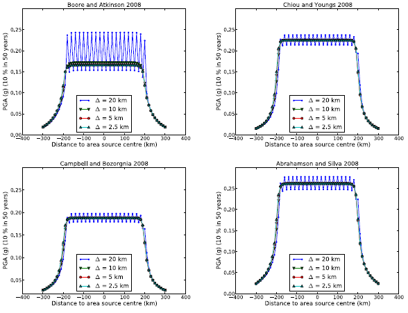
The effect of the area source discretization step :math:`(Delta)` on hazard results.#
The effect of dip and rake angles#
To investigate the effect of modelling earthquake ruptures with different inclination (that is dip angle) and faulting style (rake angle), we compare here hazard map values for an area source generating only vertical, strike-slip ruptures and an area source generating dipping (dip=50◦), reverse (rake=90◦) ruptures.
To investigate the potential dependence on the source seismic activity level, we compute hazard maps for area sources having different Gutenberg-Richter a values \(a_{GR}\) equal to 3, 4 and 5, corresponding to annual occurrence rates above M = 5 of 0.01, 0.1 and 1, respectively. Results are shown in the figure below. Sensitivity of rupture dip and faulting style clearly depends on the source activity level and on the GMPE model. Independently of the GMPE, the highest absolute difference in PGA is for the highest \(a_{GR}\). Among the different GMPE models, Campbell and Bozorgnia (2008) shows the highest sensitivity (about 20 lowest sensitivity).
The effect of the hypocentral depth distribution#
Another modeling parameter which can influence hazard estimates from an area source is the hypocentral depth distribution. We show here the effect of considering a single hypocentral depth value (10 km) versus considering a set of normally distributed values with mean µ = 10 km and standard deviation s = 4 km. By considering the same source-sites configuration as in the previous analysis, and vertical strike-slip ruptures with single strike (0◦), we compute hazard results considering two \(a_{GR}\) values (4 and 5). We use the GMPE model of Campbell and Bozorgnia (2008). the second figure below shows the computed values along the site profile for different return periods (RP) and \(a_{GR}\) values. The effect of the distribution of hypocentral values becomes visible when considering long return periods (50000 years) and increases with increasing \(a_{GR}\).
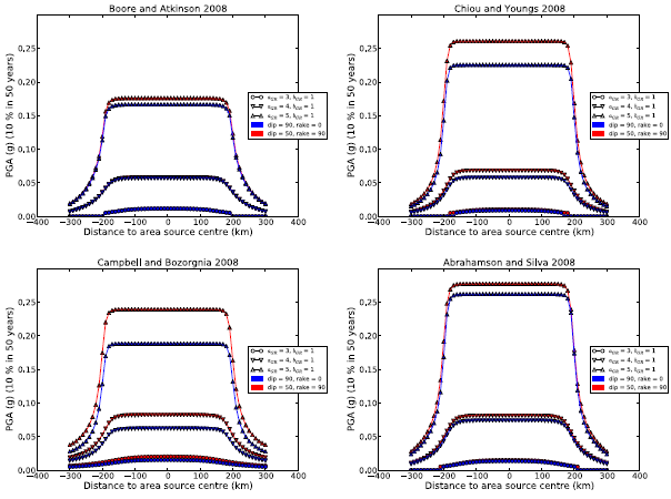
The effect of dip and rake angles on hazard results.#
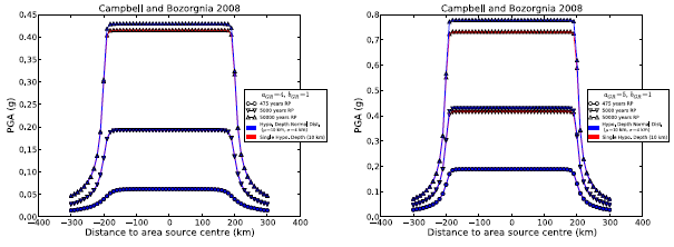
The effect of hypocentral depth on hazard map calculation.#
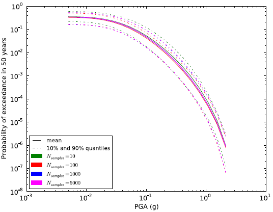
Mean and quantile hazard curves obtained from Monte Carlo sampling of logic tree.#
Classical PSHA with complex logic tree#
We consider here a synthetic case of a classical PSHA calculation based on a simple source model consisting of 5 identical area sources. Each source has a square shape of 0.5◦ side. Four sources are arranged to form a regular mesh. The fifth source is placed in the middle of the mesh and overlaps with the other four sources. Each source can have 5 possible (\(a_{GR}\), \(b_{GR}\)) pairs and 3 possible maximum magnitudes. Assuming the uncertainties to be uncorrelated among sources, the total number of possible source parameters combinations can be written as:
where \(N_{GR}\) is the number of Gutenberg-Richter parameters (i.e. \(a_{GR}\) - \(b_{GR}\) pairs) for each source, \(N_{MaxMag}\) is the number of maximum magnitudes for each source, and \(N_{S}\) is the number of sources. In the present case \(N_{GR}=5\), \(N_{MaxMag}=3\), \(N_{S}=5\), and thus \(N=5^5 \times 3^5 = 759375 N\). \(N\) represents the total number of paths in the source model logic tree.
The OpenQuake engine allows random sampling the logic tree to avoid calculating hazard results for all possible logic tree paths. The last figure above presents mean and quantile hazard curves as obtained from different numbers of samples (10, 100, 1000, 5000). It can be seen how, by increasing the number of samples, results tend to converge to similar values. Indeed, curves obtained from 1000 and 5000 samples are almost indistinguishable. The Monte Carlo sampling offers therefore an effective way to reduce the computational burden associated with a large logic tree and to still obtain reliable results. The results reliability can be controlled by performing a convergence analysis; that is by identifying the number of samples which are required to obtain values that are stable within a certain tolerance level.
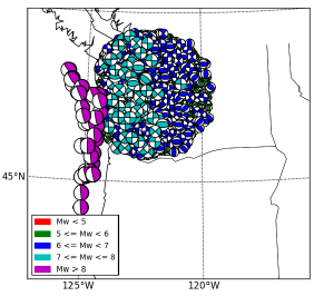
Stochastic event set for a region surrounding Seattle (U.S.) for a duration of 10000 years.#
Convergence between Classical and Event-based PSHA#
The event based approach allows generating stochastic event sets and ground motion fields which can then be used to reproduce the classical results. We present here an event-based calculation for a location corresponding to the city of Seattle. The calculation is done using the 2008 seismic hazard model for conterminous U.S. (Petersen et al., 2008). A stochastic event set covering a period of 10000 years is generated (the figure above). The event set contains earthquake ruptures within a radius of 200 km from the city of Seattle (longitude = 122.3W, latitude = 47.6N) including large subduction interface earthquakes generated in the Cascadia region, as well as deep intraslab and shallow active crust earthquakes. From each event, ground shaking values are simulated in the city of Seattle (considering the full set of GMPEs prescribed by the model). From ground motion values, the mean hazard curve (probability of exceedance in 50 years) for PGA is computed, and compared against the one obtained using the classical approach (the figure below). The curve obtained can reliably reproduce the probabilities of exceedance down to 10—2. For lower probabilities a stochastic event set with longer duration is required.
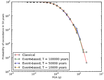
Hazard curves for Seattle using the Classical and Event-based approaches.#
Disaggregation analysis#
We present here an example of disaggregation analysis for the city of Seattle, again considering the 2008 national seismic hazard model for U.S. developed by Petersen et al. (2008). In particular, we show the geographic-magnitude (the first figure below) and geographic-tectonic region type (the second figure below) disaggregation histograms for PGA corresponding to 10% probability of exceedance in 50 years. The geographic disaggregation allows investigating the spatial distribution of the seismic sources contributing to a given level of hazard. By including magnitude and tectonic region type, we can understand the influence of the different tectonic regions, and also the magnitude ranges involved. Indeed, the disaggregation analysis for the city of Seattle shows that, for a return period of 475 years, the highest probabilities of ground motion exceedance are associated with active shallow crust events with magnitudes in the range 6 to 7. The second highest contributions are from subduction interface events with magnitudes above 9. Subduction intraslab events are instead associated to the lowest contributions.
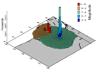
Longitude, latitude and magnitude disaggregation for PGA corresponding to 10% probability of exceedance in 50 years.#
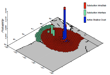
Longitude, latitude and tectonic region type disaggregation for PGA corresponding to 10% probability of exceedance in 50 years.#