1. General

This manual is for advanced users, i.e. people who already know how to use the engine and have already read the official manual cover-to-cover. If you have just started on your journey of using and working with the OpenQuake engine, this manual is probably NOT for you. Beginners should study the official manual first. This manual is intended for users who are either running large calculations or those who are interested in programatically interacting with the datastore.

For the purposes of this manual a calculation is large if it cannot be run, i.e. if it runs out of memory, it fails with strange errors or it just takes too long to complete.

There are various reasons why a calculation can be too large. 90% of the times it is because the user is making some mistakes and she is trying to run a calculation larger than she really needs. In the remaining 10% of the times the calculation is genuinely large and the solution is to buy a larger machine, or to ask the OpenQuake developers to optimize the engine for the specific calculation that is giving issues.

The first things to do when you have a large calculation is to run the command oq info --report job.ini, that will tell you essential information to estimate the size of the full calculation, in particular the number of hazard sites, the number of ruptures, the number of assets and the most relevant parameters you are using. If generating the report is slow, it means that there is something wrong with your calculation and you will never be able to run it completely unless you reduce it.

The single most important parameter in the report is the number of effective ruptures, i.e. the number of ruptures after distance and magnitude filtering. For instance your report could contain numbers like the following:

#eff_ruptures 239,556
#tot_ruptures 8,454,592

This is an example of a computation which is potentially large - there are over 8 million ruptures generated by the model - but that in practice will be very fast, since 97% of the ruptures will be filtered away. The report gives a conservative estimate, in reality even more ruptures will be discarded.

It is very common to have an unhappy combinations of parameters in the job.ini file, like discretization parameters that are too small. Then your source model with contain millions and millions of ruptures and the computation will become impossibly slow or it will run out of memory. By playing with the parameters and producing various reports, one can get an idea of how much a calculation can be reduced even before running it.

Now, it is a good time to read the section about common mistakes.

2. Common mistakes: bad configuration parameters

By far, the most common source of problems with the engine is the choice of parameters in the job.ini file. It is very easy to make mistakes, because users typically copy the parameters from the OpenQuake demos. However, the demos are meant to show off all of the features of the engine in simple calculations, they are not meant for getting performance in large calculations.

2.1. The quadratic parameters

In large calculations, it is essential to tune a few parameters that are really important. Here is a list of parameters relevant for all calculators:

maximum_distance:

The larger the maximum_distance, the more sources and ruptures will be considered; the effect is quadratic, i.e. a calculation with maximum_distance=500 km could take up to 6.25 times more time than a calculation with maximum_distance=200 km.

region_grid_spacing:

The hazard sites can be specified by giving a region and a grid step. Clearly the size of the computation is quadratic with the inverse grid step: a calculation with region_grid_spacing=1 will be up to 100 times slower than a computation with region_grid_spacing=10.

area_source_discretization:

Area sources are converted into point sources, by splitting the area region into a grid of points. The area_source_discretization (in km) is the step of the grid. The computation time is inversely proportional to the square of the discretization step, i.e. calculation with area_source_discretization=5 will take up to four times more time than a calculation with area_source_discretization=10.

rupture_mesh_spacing:

Fault sources are computed by converting the geometry of the fault into a mesh of points; the rupture_mesh_spacing is the parameter determining the size of the mesh. The computation time is quadratic with the inverse mesh spacing. Using a rupture_mesh_spacing=2 instead of rupture_mesh_spacing=5 will make your calculation up to 6.25 times slower. Be warned that the engine may complain if the rupture_mesh_spacing is too large.

complex_fault_mesh_spacing:

The same as the rupture_mesh_spacing, but for complex fault sources. If not specified, the value of rupture_mesh_spacing will be used. This is a common cause of problems; if you have performance issue you should consider using a larger complex_fault_mesh_spacing. For instance, if you use a rupture_mesh_spacing=2 for simple fault sources but complex_fault_mesh_spacing=10 for complex fault sources, your computation can become up to 25 times faster, assuming the complex fault sources are dominating the computation time.

2.2. Maximum distance

The engine gives users a lot of control on the maximum distance parameter. For instance, you can have a different maximum distance depending on the tectonic region, like in the following example:

maximum_distance = {'Active Shallow Crust': 200, 'Subduction': 500}

You can also have a magnitude-dependent maximum distance:

maximum_distance = [(5, 0), (6, 100), (7, 200), (8, 300)]

In this case, given a site, the engine will completely discard ruptures with magnitude below 5, keep ruptures up to 100 km for magnitudes between 5 and 6 (the maximum distance in this magnitude range will vary linearly between 0 and 100), keep ruptures up to 200 km for magnitudes between 6 and 7 (with maximum_distance increasing linearly from 100 to 200 km from magnitude 6 to magnitude 7), keep ruptures up to 300 km for magnitudes over 7.

You can have both trt-dependent and mag-dependent maximum distance:

maximum_distance = {
   'Active Shallow Crust': [(5, 0), (6, 100), (7, 200), (8, 300)],
   'Subduction': [(6.5, 300), (9, 500)]}

Given a rupture with tectonic region type trt and magnitude mag, the engine will ignore all sites over the maximum distance md(trt, mag). The precise value is given via linear interpolation of the values listed in the job.ini; you can determine the distance as follows:

>>> from openquake.hazardlib.calc.filters import IntegrationDistance
>>> idist = IntegrationDistance.new('[(4, 0), (6, 100), (7, 200), (8.5, 300)]')
>>> interp = idist('TRT')
>>> interp([4.5, 5.5, 6.5, 7.5, 8])
array([ 25.        ,  75.        , 150.        , 233.33333333,
       266.66666667])

2.3. pointsource_distance

PointSources (and MultiPointSources and AreaSources, which are split into PointSources and therefore are effectively the same thing) are not pointwise for the engine: they actually generate ruptures with rectangular surfaces which size is determined by the magnitude scaling relationship. The geometry and position of such rectangles depends on the hypocenter distribution and the nodal plane distribution of the point source, which are used to model the uncertainties on the hypocenter location and on the orientation of the underlying ruptures.

Is the effect of the hypocenter/nodal planes distributions relevant? Not always: in particular, if you are interested in points that are far away from the rupture the effect is minimal. So if you have a nodal plane distribution with 20 planes and a hypocenter distribution with 5 hypocenters, the engine will consider 20 x 5 ruptures and perform 100 times more calculations than needed, since at large distance the hazard will be more or less the same for each rupture.

To avoid this performance problem there is a pointsource_distance parameter: you can set it in the job.ini as a dictionary (tectonic region type -> distance in km) or as a scalar (in that case it is converted into a dictionary {"default": distance} and the same distance is used for all TRTs). For sites that are more distant than the pointsource_distance plus the rupture radius from the point source, the engine creates an average rupture by taking weighted means of the parameters strike, dip, rake and depth from the nodal plane and hypocenter distributions and by rescaling the occurrence rate. For closer points, all the original ruptures are considered. This approximation (we call it rupture collapsing because it essentially reduces the number of ruptures) can give a substantial speedup if the model is dominated by PointSources and there are several nodal planes/hypocenters in the distribution. In some situations it also makes sense to set

pointsource_distance = 0

to completely remove the nodal plane/hypocenter distributions. For instance the Indonesia model has 20 nodal planes for each point sources; however such model uses the so-called equivalent distance approximation which considers the point sources to be really pointwise. In this case the contribution to the hazard is totally independent from the nodal plane and by using pointsource_distance = 0 one can get exactly the same numbers and run the model in 1 hour instead of 20 hours. Actually, starting from engine 3.3 the engine is smart enough to recognize the cases where the equivalent distance approximation is used and automatically set pointsource_distance = 0.

Even if you not using the equivalent distance approximation, the effect of the nodal plane/hypocenter distribution can be negligible: I have seen cases when setting setting pointsource_distance = 0 changed the result in the hazard maps only by 0.1% and gained an order of magnitude of speedup. You have to check on a case by case basis.

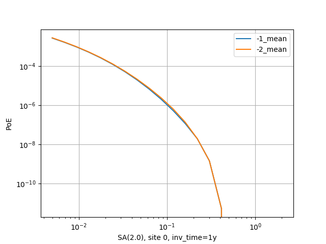
There is a good example of use of the pointsource_distance in the MultiPointClassicalPSHA demo. Here we will just show a plot displaying the hazard curve without pointsource_distance (with ID=-2) and with pointsource_distance=200 km (with ID=-1). As you see they are nearly identical but the second calculation is ten times faster.

The pointsource_distance is also crucial when using the point source gridding approximation: then it can be used to speedup calculations even when the nodal plane and hypocenter distributions are trivial and no speedup would be expected.

NB: the pointsource_distance approximation has changed a lot across engine releases and you should not expect it to give always the same results. In particular, in engine 3.8 it has been extended to take into account the fact that small magnitudes will have a smaller collapse distance. For instance, if you set pointsource_distance=100, the engine will collapse the ruptures over 100 km for the maximum magnitude, but for lower magnitudes the engine will consider a (much) shorter collapse distance and will collapse a lot more ruptures. This is possible because given a tectonic region type the engine knows all the GMPEs associated to that tectonic region and can compute an upper limit for the maximum intensity generated by a rupture at any distance. Then it can invert the curve and given the magnitude and the maximum intensity can determine the collapse distance for that magnitude.

In engine 3.11, contrarily to all previous releases, finite side effects are not ignored for distance sites, they are simply averaged over. This gives a better precision. In some case (i.e. the Alaska model) versions of the engine before 3.11 could give a completely wrong hazard on some sites. This is now fixed.

Note: setting pointsource_distance=0 does not completely remove finite size effects. If you want to replace point sources with points you need to also change the magnitude-scaling relationship to PointMSR. Then the area of the underlying planar ruptures will be set to 1E-4 squared km and the ruptures will effectively become points.

2.4. The linear parameters: width_of_mfd_bin and intensity levels

The number of ruptures generated by the engine is controlled by the parameter width_of_mfd_bin; for instance if you raise it from 0.1 to 0.2 you will reduce by half the number of ruptures and double the speed of the calculation. It is a linear parameter, at least approximately. Classical calculations are also roughly linear in the number of intensity measure types and levels. A common mistake is to use too many levels. For instance a configuration like the following one:

intensity_measure_types_and_levels = {
  "PGA":  logscale(0.001,4.0, 100),
  "SA(0.3)":  logscale(0.001,4.0, 100),
  "SA(1.0)":  logscale(0.001,4.0, 100)}

requires computing the PoEs on 300 levels. Is that really what the user wants? It could very well be that using only 20 levels per each intensity measure type produces good enough results, while potentially reducing the computation time by a factor of 5.

2.5. concurrent_tasks parameter

There is a last parameter which is worthy of mention, because of its effect on the memory occupation in the risk calculators and in the event based hazard calculator.

concurrent_tasks:

This is a parameter that you should not set, since in most cases the engine will figure out the correct value to use. However, in some cases, you may be forced to set it. Typically this happens in event based calculations, when computing the ground motion fields. If you run out of memory, increasing this parameter will help, since the engine will produce smaller tasks. Another case when it may help is when computing hazard statistics with lots of sites and realizations, since by increasing this parameter the tasks will contain less sites.

Notice that if the number of concurrent_tasks is too big the performance will get worse and the data transfer will increase: at a certain point the calculation will run out of memory. I have seen this to happen when generating tens of thousands of tasks. Again, it is best not to touch this parameter unless you know what you are doing.

3. Developing with the engine

Some advanced users are interested in developing with the engine, usually to contribute new GMPEs and sometimes to submit a bug fix. There are also users interested in implementing their own customizations of the engine. This part of the manual is for them.

3.1. Prerequisites

It is assumed here that you are a competent scientific Python programmer, i.e. that you have a good familiarity with the Python ecosystem (including pip and virtualenv) and its scientific stack (numpy, scipy, h5py, …). It should be noticed that since engine v2.0 there is no need to know anything about databases and web development (unless you want to develop on the WebUI part) so the barrier for contribution to the engine is much lower than it used to be. However, contributing is still nontrivial, and it absolutely necessary to know git and the tools of Open Source development in general, in particular about testing. If this is not the case, you should do some study on your own and come back later. There is a huge amount of resources on the net about these topics. This manual will focus solely on the OpenQuake engine and it assume that you already know how to use it, i.e. you have read the User Manual first.

Before starting, it may be useful to have an idea of the architecture of the engine and its internal components, like the DbServer and the WebUI. For that you should read the Architecture of the OpenQuake engine document.

There are also external tools which are able to interact with the engine, like the QGIS plugin to run calculations and visualize the outputs and the IPT tool to prepare the required input files (except the hazard models). Unless you are developing for such tools you can safely ignore them.

3.2. The first thing to do

The first thing to do if you want to develop with the engine is to remove any non-development installation of the engine that you may have. While it is perfectly possible to install on the same machine both a development and a production instance of the engine (it is enough to configure the ports of the DbServer and WebUI) it is easier to work with a single instance. In that way you will have a single code base and no risks of editing the wrong code. A development installation the engine works as any other development installation in Python: you should clone the engine repository, create and activate a virtualenv and then perform a pip install -e . from the engine main directory, as normal. You can find the details here:

gem/oq-engine

It is also possible to develop on Windows ( gem/oq-engine) but very few people in GEM are doing that, so you are on your own, should you encounter difficulties. We recommend Linux, but Mac also works.

Since you are going to develop with the engine, you should also install the development dependencies that by default are not installed. They are listed in the setup.py file, and currently (January 2020) they are pytest, flake8, pdbpp, silx and ipython. They are not required but very handy and recommended. It is the stack we use daily for development.

3.3. Understanding the engine

Once you have the engine installed you can run calculations. We recommend starting from the demos directory which contains example of hazard and risk calculations. For instance you could run the area source demo with the following command:

$ oq run demos/hazard/AreaSourceClassicalPSHA/job.ini

You should notice that we used here the command oq run while the engine manual recommend the usage of oq engine --run. There is no contradiction. The command oq engine --run is meant for production usage, but here we are doing development, so the recommended command is oq run which will will be easier to debug thanks to the flag --pdb, which will start the python debugger should the calculation fail. Since during development is normal to have errors and problems in the calculation, this ability is invaluable.

If you want to understand what happened during the calculation you should generate the associated .rst report, which can be seen with the command

$ oq show fullreport

There you will find a lot of interesting information that it is worth studying and we will discuss in detail in the rest of this manual. The most important section of the report is probably the last one, titled “Slowest operations”. For that one can understand the bottlenecks of a calculation and, with experience, he can understand which part of the engine he needs to optimize. Also, it is very useful to play with the parameters of the calculation (like the maximum distance, the area discretization, the magnitude binning, etc etc) and see how the performance change. There is also a command to plot hazard curves and a command to compare hazard curves between different calculations: it is common to be able to get big speedups simply by changing the input parameters in the job.ini of the model, without changing much the results.

There a lot of oq commands: if you are doing development you should study all of them. They are documented here.

3.4. Running calculations programmatically

Starting from engine 3.12 the recommended way to run a job programmaticaly is the following:

>> from openquake.commonlib import logs
>> from openquake.calculators.base import calculators
>> with logs.init('job', 'job_ini') as log: # initialize logs
...   calc = calculators(log.get_oqparam(), log.calc_id)
...   calc.run()  # run the calculator

Then the results can be read from the datastore by using the extract API:

>> from openquake.calculators.extract import extract
>> extract(calc.datastore, 'something')

3.5. Case study: computing the impact of a source on a site

As an exercise showing off how to use the engine as a library, we will solve the problem of computing the hazard on a given site generated by a given source, with a given GMPE logic tree and a few parameters, i.e. the intensity measure levels and the maximum distance.

The first step is to specify the site and the parameters; let’s suppose that we want to compute the probability of exceeding a Peak Ground Accelation (PGA) of 0.1g by using the ToroEtAl2002SHARE GMPE:

>>> from openquake.commonlib import readinput
>>> oq = readinput.get_oqparam(dict(
... calculation_mode='classical',
... sites='15.0 45.2',
... reference_vs30_type='measured',
... reference_vs30_value='600.0',
... intensity_measure_types_and_levels="{'PGA': [0.1]}",
... investigation_time='50.0',
... gsim='ToroEtAl2002SHARE',
... maximum_distance='200.0'))

Then we need to specify the source:

>>> from openquake.hazardlib import nrml
>>> src = nrml.get('''
...         <areaSource
...         id="126"
...         name="HRAS195"
...         >
...             <areaGeometry discretization="10">
...                 <gml:Polygon>
...                     <gml:exterior>
...                         <gml:LinearRing>
...                             <gml:posList>
...                                 1.5026169E+01 4.5773603E+01
...                                 1.5650548E+01 4.6176279E+01
...                                 1.6273108E+01 4.6083465E+01
...                                 1.6398742E+01 4.6024744E+01
...                                 1.5947759E+01 4.5648318E+01
...                                 1.5677179E+01 4.5422577E+01
...                             </gml:posList>
...                         </gml:LinearRing>
...                     </gml:exterior>
...                 </gml:Polygon>
...                 <upperSeismoDepth>0</upperSeismoDepth>
...                 <lowerSeismoDepth>30</lowerSeismoDepth>
...             </areaGeometry>
...             <magScaleRel>WC1994</magScaleRel>
...             <ruptAspectRatio>1</ruptAspectRatio>
...             <incrementalMFD binWidth=".2" minMag="4.7">
...                 <occurRates>
...                     1.4731083E-02 9.2946848E-03 5.8645496E-03
...                     3.7002807E-03 2.3347193E-03 1.4731083E-03
...                     9.2946848E-04 5.8645496E-04 3.7002807E-04
...                     2.3347193E-04 1.4731083E-04 9.2946848E-05
...                     1.7588460E-05 1.1097568E-05 2.3340307E-06
...                 </occurRates>
...             </incrementalMFD>
...             <nodalPlaneDist>
...                 <nodalPlane dip="5.7596810E+01" probability="1"
...                             rake="0" strike="6.9033586E+01"/>
...             </nodalPlaneDist>
...             <hypoDepthDist>
...                 <hypoDepth depth="1.0200000E+01" probability="1"/>
...             </hypoDepthDist>
...         </areaSource>
... ''')

Then the hazard curve can be computed as follows:

>>> from openquake.hazardlib.calc.hazard_curve import calc_hazard_curve
>>> from openquake.hazardlib import valid
>>> sitecol = readinput.get_site_collection(oq)
>>> gsims = readinput.get_gsim_lt(oq).values['*']
>>> calc_hazard_curve(sitecol, src, gsims, oq)
<ProbabilityCurve
[[0.00507997]]>

3.6. Working with GMPEs directly: the ContextMaker

If you are an hazard scientist, you will likely want to interact with the GMPE library in openquake.hazardlib.gsim. The recommended way to do so is in terms of a ContextMaker object.

>>> from openquake.hazardlib.contexts import ContextMaker

In order to instantiate a ContextMaker you first need to populate a dictionary of parameters:

>>> param = dict(maximum_distance=oq.maximum_distance, imtls=oq.imtls,
...              truncation_level=oq.truncation_level,
...              investigation_time=oq.investigation_time)
>>> cmaker = ContextMaker(src.tectonic_region_type, gsims, param)

Then you can use the ContextMaker to generate context arrays from the sources:

>>> [ctx] = cmaker.from_srcs([src], sitecol)

In our example, there are 15 magnitudes

>>> len(src.get_annual_occurrence_rates())
15

and the area source contains 47 point sources

>>> len(list(src))
47

so in total there are 15 x 47 = 705 ruptures:

>>> len(ctx)
705

The ContextMaker takes care of the maximum_distance filtering, so in general the number of contexts is lower than the total number of ruptures, since some ruptures are normally discarded, being distant from the sites.

The contexts contains all the rupture, site and distance parameters.

Then you have

>>> ctx.mag[0]
4.7
>>> round(ctx.rrup[0], 1)
106.4
>>> round(ctx.rjb[0], 1)
105.9

In this example, the GMPE ToroEtAl2002SHARE does not require site parameters, so calling ctx.vs30 will raise an AttributeError but in general the contexts contains also arrays of site parameters. There is also an array of indices telling which are the sites affected by the rupture associated to the context:

>>> import numpy
>>> numpy.unique(ctx.sids)
array([0], dtype=uint32)

Once you have the contexts, the ContextMaker is able to compute means and standard deviations from the underlying GMPEs as follows (for engine version >= 3.13):

>>> mean, sig, tau, phi = cmaker.get_mean_stds([ctx])

Since in this example there is a single gsim and a single IMT you will get:

>>> mean.shape
(1, 1, 705)
>>> sig.shape
(1, 1, 705)

The shape of the arrays in general is (G, M, N) where G is the number of GSIMs, M the number of intensity measure types and N the total size of the contexts. Since this is an example with a single site, each context has size 1, therefore N = 705 * 1 = 705. In general if there are multiple sites a context M is the total number of affected sites. For instance if there are two contexts and the first affect 1 sites and the second 2 sites then N would be 1 + 2 = 3. This example correspond to 1 + 1 + … + 1 = 705.

From the mean and standard deviation is possible to compute the probabilities of exceedence. The ContextMaker provides a method to compute directly the probability map, which internally calls `cmaker.get_pmap([ctx]) which gives exactly the result provided by calc_hazard_curve(sitecol, src, gsims, oq) in the section before.

If you want to know exactly how get_pmap works you are invited to look at the source code in openquake.hazardlib.contexts.

3.7. Working with verification tables

Hazard scientists implementing a new GMPE must provide verification tables, i.e. CSV files containing inputs and expected outputs.

For instance, for the Atkinson2015 GMPE (chosen simply because is the first GMPE in lexicographic order in hazardlib) the verification table has a structure like this:

rup_mag,dist_rhypo,result_type,pgv,pga,0.03,0.05,0.1,0.2,0.3,0.5
2.0,1.0,MEAN,5.50277734e-02,3.47335058e-03,4.59601700e-03,7.71361460e-03,9.34624779e-03,4.33207607e-03,1.75322233e-03,3.44695521e-04
2.0,5.0,MEAN,6.43850933e-03,3.61047741e-04,4.57949482e-04,7.24558049e-04,9.44495571e-04,5.11252304e-04,2.21076069e-04,4.73435138e-05
...

The columns starting with rup_ contains rupture parameters (the magnitude in this example) while the columns starting with dist_ contains distance parameters. The column result_type is a string in the set {“MEAN”, “INTER_EVENT_STDDEV”, “INTRA_EVENT_STDDEV”, “TOTAL_STDDEV”}. The remaining columns are the expected results for each intensity measure type; in the the example the IMTs are PGV, PGA, SA(0.03), SA(0.05), SA(0.1), SA(0.2), SA(0.3), SA(0.5).

Starting from engine version 3.13, it is possible to instantiate a ContextMaker and the associated contexts from a GMPE and its verification tables with a few simple steps. First of all one must instantiate the GMPE:

>>> from openquake.hazardlib import valid
>>> gsim = valid.gsim("Atkinson2015")

Second, one can determine the path names to the verification tables as follows (they are in a subdirectory of hazardlib/tests/gsim/data):

>>> import os
>>> from openquake.hazardlib.tests.gsim import data
>>> datadir = os.path.join(data.__path__[0], 'ATKINSON2015')
>>> fnames = [os.path.join(datadir, f) for f in ["ATKINSON2015_MEAN.csv",
...           "ATKINSON2015_STD_INTER.csv", "ATKINSON2015_STD_INTRA.csv",
...           "ATKINSON2015_STD_TOTAL.csv"]]

Then it is possible to instantiate the ContextMaker associated to the GMPE and a pandas DataFrame associated to the verification tables in a single step:

>>> from openquake.hazardlib.tests.gsim.utils import read_cmaker_df, gen_ctxs
>>> cmaker, df = read_cmaker_df(gsim, fnames)
>>> list(df.columns)
['rup_mag', 'dist_rhypo', 'result_type', 'damping', 'PGV', 'PGA', 'SA(0.03)', 'SA(0.05)', 'SA(0.1)', 'SA(0.2)', 'SA(0.3)', 'SA(0.5)', 'SA(1.0)', 'SA(2.0)', 'SA(3.0)', 'SA(5.0)']

Then you can immediately compute mean and standard deviations and compare with the values in the verification table:

>>> mean, sig, tau, phi = cmaker.get_mean_stds(gen_ctxs(df))

sig refers to the “TOTAL_STDDEV”, tau to the “INTER_EVENT_STDDEV” and phi to the “INTRA_EVENT_STDDEV”. This is how the tests in hazardlib are implemented. Interested users should look at the code in gem/oq-engine.

3.8. Running the engine tests

If you are a hazard scientists contributing a bug fix to a GMPE (or any other kind of bug fix) you may need to run the engine tests and possibly change the expected files if there is a change in the numbers. The way to do it is to start the dbserver and then run the tests from the repository root:

$ oq dbserver start
$ pytest -vx openquake/calculators

If you get an error like the following:

openquake/calculators/tests/__init__.py:218: in assertEqualFiles
    raise DifferentFiles('%s %s' % (expected, actual))
E   openquake.calculators.tests.DifferentFiles: /home/michele/oq-engine/openquake/qa_tests_data/classical/case_1/expected/hazard_curve-PGA.csv /tmp/tmpkdvdhlq5/hazard_curve-mean-PGA_27249.csv

you need to change the expected file, i.e. copy the file /tmp/tmpkdvdhlq5/hazard_curve-mean-PGA_27249.csv over classical/case_1/expected/hazard_curve-PGA.csv.

4. Architecture of the OpenQuake engine

The engine is structured as a regular scientific application: we try to perform calculations as much as possible in memory and when it is not possible intermediate results are stored in HDF5 format. We try work as much as possible in terms of arrays which are efficiently manipulated at C/Fortran speed with a stack of well established scientific libraries (numpy/scipy).

CPU-intensity calculations are parallelized with a custom framework (the engine is ten years old and predates frameworks like dask or ray) which however is quite easy to use and mostly compatible with Python multiprocessing or concurrent.futures. The concurrency architecture is the standard Single Writer Multiple Reader (SWMR), used at the HDF5 level: only one process can write data while multiple processes can read it. The engine runs seamlessly on a single machine or a cluster, using as many cores as possible.

In the past the engine had a database-centric architecture and was more class-oriented than numpy-oriented: some remnants of such dark past are still there, but they are slowly disappearing. Currently the database is only used for storing accessory data and it is a simple SQLite file. It is mainly used by the WebUI to display the logs.

4.1. Components of the OpenQuake Engine

The OpenQuake Engine suite is composed of several components:

• a set of support libraries addressing different concerns like reading the inputs and writing the outputs, implementing basic geometric manipulations, managing distributed computing and generic programming utilities

• the hazardlib and risklib scientific libraries, providing the building blocks for hazard and risk calculations, notably the GMPEs for hazard and the vulnerability/fragility functions for risk

• the hazard and risk calculators, implementing the core logic of the engine

• the datastore, which is an HDF5 file working as a short term storage/cache for a calculation; it is possible to run a calculation starting from an existing datastore, to avoid recomputing everything every time; there is a separate datastore for each calculation

• the database, which is a SQLite file working as a long term storage for the calculation metadata; the database contains the start/stop times of the computations, the owner of a calculation, the calculation descriptions, the performances, the logs, etc; the bulk scientific data (essentially big arrays) are kept in the datastore

• the DbServer, which is a service mediating the interaction between the calculators and the database

• the WebUI is a web application that allows to run and monitor computations via a browser; multiple calculations can be run in parallel

• the oq command-line tool; it allows to run computations and provides an interface to the underlying database and datastores so that it is possible to list and export the results

• the engine can run on a cluster of machines: in that case a minimal amount of configuration is needed, whereas in single machine installations the engine works out of the box

• since v3.8 the engine does not depend anymore from celery and rabbitmq, but can still use such tools until they will be deprecated

This is the full stack of internal libraries used by the engine. Each of these is a Python package containing several modules or event subpackages. The stack is a dependency tower where the higher levels depend on the lower levels but not vice versa:

• level 9: commands (subcommands of oq)

• level 8: server (database and Web UI)

• level 7: engine (command-line tool, export, logs)

• level 6: calculators (hazard and risk calculators)

• level 5: commonlib (configuration, logic trees, I/O)

• level 4: risklib (risk validation, risk models, risk inputs)

• level 3: hmtk (catalogues, plotting, …)

• level 2: hazardlib (validation, read/write XML, source and site objects, geospatial utilities, GSIM library)

• level 1: baselib (programming utilities, parallelization, monitoring, hdf5…)

baselib and hazardlib are very stable and can be used outside of the engine; the other libraries are directly related to the engine and are likely to be affected by backward-incompatible changes in the future, as the code base evolves.

The GMPE library in hazardlib and the calculators are designed to be extensible, so that it is easy to add a new GMPE class or a new calculator. We routinely add several new GMPEs per release; adding new calculators is less common and it requires more expertise, but it is possible and it has been done several times in the past. In particular it is often easier to add a specific calculator optimized for a given use case rather than complicating the current calculators.

The results of a computation are automatically saved in the datastore and can be exported in a portable format, such as CSV (or XML, for legacy reasons). You can assume that the datastore of version X of the engine will not work with version X + 1. On the contrary, the exported files will likely be same across different versions. It is important to export all of the outputs you are interested in before doing an upgrade, otherwise you would be forced to downgrade in order to be able to export the previous results.

The WebUI provides a REST API that can be used in third party applications: for instance a QGIS plugin could download the maps generated by the engine via the WebUI and display them. There is lot of functionality in the API which is documented here: gem/oq-engine. It is possible to build your own user interface for the engine on top of it, since the API is stable and kept backward compatible.

4.2. Design principles

The main design principle has been simplicity: everything has to be as simple as possible (but not simplest). The goal has been to keep the engine simple enough that a single person can understand it, debug it, and extend it without tremendous effort. All the rest comes from simplicity: transparency, ability to inspect and debug, modularity, adaptability of the code, etc. Even efficiency: in the last three years most of the performance improvements came from free, just from removing complications. When a thing is simple it is easy to make it fast. The battle for simplicity is never ending, so there are still several things in the engine that are more complex than they should: we are working on that.

After simplicity the second design goal has been performance: the engine is a number crunching application after all, and we need to run massively parallel calculations taking days or weeks of runtime. Efficiency in terms of computation time and memory requirements is of paramount importance, since it makes the difference between being able to run a computation and being unable to do it. Being too slow to be usable should be considered as a bug.

The third requirement is reproducibility, which is the same as testability: it is essential to have a suite of tests checking that the calculators are providing the expected outputs against a set of predefined inputs. Currently we have thousands of tests which are run multiple times per day in our Continuous Integration environments r(avis, GitLab, Jenkins), split into unit tests, end-to-end tests and long running tests.

5. How the parallelization works in the engine

The engine builds on top of existing parallelization libraries. Specifically, on a single machine it is based on multiprocessing, which is part of the Python standard library, while on a cluster it is based on the combination celery/rabbitmq, which are well-known and maintained tools.

While the parallelization used by the engine may look trivial in theory (it only addresses embarrassingly parallel problems, not true concurrency) in practice it is far from being so. For instance a crucial feature that the GEM staff requires is the ability to kill (revoke) a running calculation without affecting other calculations that may be running concurrently.

Because of this requirement, we abandoned concurrent.futures, which is also in the standard library, but is lacking the ability to kill the pool of processes, which is instead available in multiprocessing with the Pool.shutdown method. For the same reason, we discarded dask, which is a lot more powerful than celery but lacks the revoke functionality.

Using a real cluster scheduling mechanism (like SLURM) would be of course better, but we do not want to impose on our users a specific cluster architecture. celery/rabbitmq have the advantage of being simple to install and manage. Still, the architecture of the engine parallelization library is such that it is very simple to replace celery/rabbitmq with other parallelization mechanisms: people interested in doing so should just contact us.

Another tricky aspects of parallelizing large scientific calculations is that the amount of data returned can exceed the 4 GB limit of Python pickles: in this case one gets ugly runtime errors. The solution we found is to make it possible to yield partial results from a task: in this way instead of returning say 40 GB from one task, one can yield 40 times partial results of 1 GB each, thus bypassing the 4 GB limit. It is up to the implementor to code the task carefully. In order to do so, it is essential to have in place some monitoring mechanism measuring how much data is returned back from a task, as well as other essential informations like how much memory is allocated and how long it takes to run a task.

To this aim the OpenQuake engine offers a Monitor class (located in openquake.baselib.performance) which is perfectly well integrated with the parallelization framework, so much that every task gets a Monitor object, a context manager that can be used to measure time and memory of specific parts of a task. Moreover, the monitor automatically measures time and memory for the whole task, as well as the size of the returned output (or outputs). Such information is stored in an HDF5 file that you must pass to the monitor when instantiating it. The engine automatically does that for you by passing the pathname of the datastore.

In OpenQuake a task is just a Python function (or generator) with positional arguments, where the last argument is a Monitor instance. For instance the rupture generator task in an event based calculation is coded more or less like this:

def sample_ruptures(sources, num_samples, monitor):  # simplified code
    ebruptures = []
    for src in sources:
        for rup, n_occ in src.sample_ruptures(num_samples):
            ebr = EBRupture(rup, src.id, grp_id, n_occ)
            eb_ruptures.append(ebr)
        if len(eb_ruptures) > MAX_RUPTURES:
            # yield partial result to avoid running out of memory
            yield eb_ruptures
            eb_ruptures.clear()
    if ebruptures:
        yield eb_ruptures

If you know that there is no risk of running out of memory and/or passing the pickle limit you can just use a regular function and return a single result instead of yielding partial results. This is the case when computing the hazard curves, because the algorithm is considering one rupture at the time and it is not accumulating ruptures in memory, differently from what happens when sampling the ruptures in event based.

If you have ever coded in celery, you will see that the OpenQuake engine concept of task is different: there is no @task decorator and while at the end engine tasks will become celery tasks this is hidden to the developer. The reason is that we needed a celery-independent abstraction layer to make it possible to use different kinds of parallelization frameworks/

From the point of view of the coder, in the engine there is no difference between a task running on a cluster using celery and a task running locally using multiprocessing.Pool: they are coded the same, but depending on a configuration parameter in openquake.cfg (distribute=celery or distribute=processpool) the engine will treat them differently. You can also set an environment variable OQ_DISTRIBUTE, which takes the precedence over openquake.cfg, to specify which kind of distribution you want to use (celery or processpool): this is mostly used when debugging, when you typically insert a breakpoint in the task and then run the calculation with

$ OQ_DISTRIBUTE=no oq run job.ini

no is a perfectly valid distribution mechanism in which there is actually no distribution and all the tasks run sequentially in the same core. Having this functionality is invaluable for debugging.

Another tricky bit of real life parallelism in Python is that forking does not play well with the HDF5 library: so in the engine we are using multiprocessing in the spawn mode, not in fork mode: fortunately this feature has become available to us in Python 3 and it made our life a lot happier. Before it was extremely easy to incur unspecified behavior, meaning that reading an HDF5 file from a forked process could

1. work perfectly well

2. read bogus numbers

3. cause a segmentation fault

and all of the three things could happen unpredictably at any moment, depending on the machine where the calculation was running, the load on the machine, and any kind of environmental circumstances.

Also, while with the newest HDF5 libraries it is possible to use a Single Writer Multiple Reader architecture (SWMR), and we are actually using it - even if it is sometimes tricky to use it correctly - the performance is not always good. So, when it matters, we are using a two files approach which is simple and very effective: we read from one file (with multiple readers) and we write on the other file (with a single writer). This approach bypasses all the limitations of the SWMR mode in HDF5 and did not require a large refactoring of our existing code.

Another tricky point in cluster situations is that rabbitmq is not good at transferring gigabytes of data: it was meant to manage lots of small messages, but here we are perverting it to manage huge messages, i.e. the large arrays coming from a scientific calculations.

Hence, since recent versions of the engine we are no longer returning data from the tasks via celery/rabbitmq: instead, we use zeromq. This is hidden from the user, but internally the engine keeps track of all tasks that were submitted and waits until they send the message that they finished. If one tasks runs out of memory badly and never sends the message that it finished, the engine may hang, waiting for the results of a task that does not exist anymore. You have to be careful. What we did in our cluster is to set some memory limit on the celery user with the cgroups technology, so that an out of memory task normally fails in a clean way with a Python MemoryError, sends the message that it finished and nothing particularly bad happens. Still, in situations of very heavy load the OOM killer may enter in action aggressively and the main calculation may hang: in such cases you need a good sysadmin having put in place some monitor mechanism, so that you can see if the OOM killer entered in action and then you can kill the main process of the calculation by hand. There is not much more that can be done for really huge calculations that stress the hardware as much as possible. You must be prepared for failures.

5.1. How to use openquake.baselib.parallel

Suppose you want to code a character-counting algorithm, which is a textbook exercise in parallel computing and suppose that you want to store information about the performance of the algorithm. Then you should use the OpenQuake Monitor class, as well as the utility openquake.baselib.commonlib.hdf5new that build an empty datastore for you. Having done that, the openquake.baselib.parallel.Starmap class can take care of the parallelization for you as in the following example:

import os
import sys
import pathlib
import collections
from openquake.baselib.performance import Monitor
from openquake.baselib.parallel import Starmap
from openquake.commonlib.datastore import hdf5new


def count(text):
    c = collections.Counter()
    for word in text.split():
        c += collections.Counter(word)
    return c


def main(dirname):
    dname = pathlib.Path(dirname)
    with hdf5new() as hdf5:  # create a new datastore
        monitor = Monitor('count', hdf5)  # create a new monitor
        iterargs = ((open(dname/fname, encoding='utf-8').read(),)
                    for fname in os.listdir(dname)
                    if fname.endswith('.rst'))  # read the docs
        c = collections.Counter()  # intially empty counter
        for counter in Starmap(count, iterargs, monitor):
            c += counter
        print(c)  # total counts
        print('Performance info stored in', hdf5)


if __name__ == '__main__':
    main(sys.argv[1])  # pass the directory where the .rst files are

The name Starmap was chosen it looks very similar to multiprocessing.Pool.starmap works, the only apparent difference being in the additional monitor argument:

pool.starmap(func, iterargs) ->  Starmap(func, iterargs, monitor)

In reality the Starmap has a few other differences:

1. it does not use the multiprocessing mechanism to returns back the results, it uses zmq instead;

2. thanks to that, it can be extended to generator functions and can yield partial results, thus overcoming the limitations of multiprocessing

3. the Starmap has a .submit method and it is actually more similar to concurrent.futures than to multiprocessing.

Here is how you would write the same example by using .submit:

def main(dirname):
    dname = pathlib.Path(dirname)
    with hdf5new() as hdf5:
        smap = Starmap(count, monitor=Monitor('count', hdf5))
        for fname in os.listdir(dname):
            if fname.endswith('.rst'):
                smap.submit(open(dname/fname, encoding='utf-8').read())
        c = collections.Counter()
        for counter in smap:
            c += counter

The difference with concurrent.futures is that the Starmap takes care for of all submitted tasks, so you do not need to use something like concurrent.futures.completed, you can just loop on the Starmap object to get the results from the various tasks.

The .submit approach is more general: for instance you could define more than one Starmap object at the same time and submit some tasks with a starmap and some others with another starmap: this may help parallelizing complex situations where it is expensive to use a single starmap. However, there is limit on the number of starmaps that can be alive at the same moment.

Moreover the Starmap has a .shutdown methods that allows to shutdown the underlying pool.

The idea is to submit the text of each file - here I am considering .rst files, like the ones composing this manual - and then loop over the results of the Starmap. This is very similar to how concurrent.futures works.

6. Extracting data from calculations

The engine has a relatively large set of predefined outputs, that you can get in various formats, like CSV, XML or HDF5. They are all documented in the manual and they are the recommended way of interacting with the engine, if you are not tech-savvy.

However, sometimes you must be tech-savvy: for instance if you want to post-process hundreds of GB of ground motion fields produced by an event based calculation, you should not use the CSV output, at least if you care about efficiency. To manage this case (huge amounts of data) there a specific solution, which is also able to manage the case of data lacking a predefined exporter: the Extractor API.

There are actually two different kind of extractors: the simple Extractor, which is meant to manage large data sets (say > 100 MB) and the WebExtractor, which is able to interact with the WebAPI and to extract data from a remote machine. The WebExtractor is nice, but cannot be used for large amount of data for various reasons; in particular, unless your Internet connection is ultra-fast, downloading GBs of data will probably send the web request in timeout, causing it to fail. Even if there is no timeout, the WebAPI will block, everything will be slow, the memory occupation and disk space will go up, and at certain moment something will fail.

The WebExtractor is meant for small to medium outputs, things like the mean hazard maps - an hazard map containing 100,000 points and 3 PoEs requires only 1.1 MB of data at 4 bytes per point. Mean hazard curves or mean average losses in risk calculation are still small enough for the WebExtractor. But if you want to extract all of the realizations you must go with the simple Extractor: in that case your postprocessing script must run in the remote machine, since it requires direct access to the datastore.

Here is an example of usage of the Extractor to retrieve mean hazard curves:

>> from openquake.calculators.extract import Extractor
>> calc_id = 42  # for example
>> extractor = Extractor(calc_id)
>> obj = extractor.get('hcurves?kind=mean&imt=PGA')  # returns an ArrayWrapper
>> obj.mean.shape  # an example with 10,000 sites and 20 levels per PGA
(10000, 1, 20)
>> extractor.close()

If in the calculation you specified the flag individual\_rlzs=true, then it is also possible to retrieve a specific realization

>> dic = vars(extractor.get('hcurves?kind=rlz-0'))
>> dic['rlz-000']  # array of shape (num_sites, num_imts, num_levels)

or even all realizations:

>> dic = vars(extractor.get('hcurves?kind=rlzs'))

Here is an example of using the WebExtractor to retrieve hazard maps. Here we assumes that there is available in a remote machine where there is a WebAPI server running, a.k.a. the Engine Server. The first thing to is to set up the credentials to access the WebAPI. There are two cases:

1. you have a production installation of the engine in /opt

2. you have a development installation of the engine in a virtualenv

In both case you need to create a file called openquake.cfg with the following format:

[webapi]
server = http(s)://the-url-of-the-server(:port)
username = my-username
password = my-password

username and password can be left empty if the authentication is not enabled in the server, which is the recommended way, if the server is in your own secure LAN. Otherwise you must set the right credentials. The difference between case 1 and case 2 is in where to put the openquake.cfg file: if you have a production installation, put it in your $HOME, if you have a development installation, put it in your virtualenv directory.

The usage then is the same as the regular extractor:

>> from openquake.calculators.extract import WebExtractor
>> extractor = WebExtractor(calc_id)
>> obj = extractor.get('hmaps?kind=mean&imt=PGA')  # returns an ArrayWrapper
>> obj.array.shape  # an example with 10,000 sites and 4 PoEs
(10000, 4)
>> extractor.close()

If you do not want to put your credentials in the openquake.cfg file, you can do so, but then you need to pass them explicitly to the WebExtractor:

>> extractor = WebExtractor(calc_id, server, username, password)

6.1. Plotting

The (Web)Extractor is used in the oq plot command: by configuring openquake.cfg it is possible to plot things like hazard curves, hazard maps and uniform hazard spectra for remote (or local) calculations. Here are three examples of use:

$ oq plot 'hcurves?kind=mean&imt=PGA&site_id=0' <calc_id>
$ oq plot 'hmaps?kind=mean&imt=PGA' <calc_id>
$ oq plot 'uhs?kind=mean&site_id=0' <calc_id>

The site_id is optional; if missing only the first site (site_id=0) will be plotted. If you want to plot all the realizations you can do:

$ oq plot 'hcurves?kind=rlzs&imt=PGA' <calc_id>

If you want to plot all statistics you can do:

$ oq plot 'hcurves?kind=stats&imt=PGA' <calc_id>

It is also possible to combine plots. For instance if you want to plot all realizations and also the mean the command to give is:

$ oq plot 'hcurves?kind=rlzs&kind=mean&imt=PGA' <calc_id>

If you want to plot the mean and the median the command is:

$ oq plot 'hcurves?kind=quantile-0.5&kind=mean&imt=PGA' <calc_id>

assuming the median (i.e. quantile-0.5) is available in the calculation. If you want to compare say rlz-0 with rlz-2 and rlz-5 you can just just say so:

$ oq plot 'hcurves?kind=rlz-0&kind=rlz-2&kind=rlz-5&imt=PGA' <calc_id>

You can combine as many kinds of curves as you want. Clearly if your are specifying a kind that is not available you will get an error.

6.2. Extracting ruptures

Here is an example for the event based demo:

$ cd oq-engine/demos/hazard/EventBasedPSHA/
$ oq engine --run job.ini
$ oq shell
IPython shell with a global object "o"
In [1]: from openquake.calculators.extract import Extractor
In [2]: extractor = Extractor(calc_id=-1)
In [3]: aw = extractor.get('rupture_info?min_mag=5')
In [4]: aw
Out[4]: <ArrayWrapper(1511,)>
In [5]: aw.array
Out[5]:
array([(   0, 1, 5.05, 0.08456118,  0.15503392, 5., b'Active Shallow Crust', 0.0000000e+00, 90.      , 0.),
       (   1, 1, 5.05, 0.08456119,  0.15503392, 5., b'Active Shallow Crust', 4.4999969e+01, 90.      , 0.),
       (   2, 1, 5.05, 0.08456118,  0.15503392, 5., b'Active Shallow Crust', 3.5999997e+02, 49.999985, 0.),
       ...,
       (1508, 2, 6.15, 0.26448786, -0.7442877 , 5., b'Active Shallow Crust', 0.0000000e+00, 90.      , 0.),
       (1509, 1, 6.15, 0.26448786, -0.74428767, 5., b'Active Shallow Crust', 2.2499924e+02, 50.000004, 0.),
       (1510, 1, 6.85, 0.26448786, -0.74428767, 5., b'Active Shallow Crust', 4.9094699e-04, 50.000046, 0.)],
      dtype=[('rup_id', '<u4'), ('multiplicity', '<u2'), ('mag', '<f4'), ('centroid_lon', '<f4'),
             ('centroid_lat', '<f4'), ('centroid_depth', '<f4'), ('trt', 'S50'), ('strike', '<f4'),
             ('dip', '<f4'), ('rake', '<f4')])
In [6]: extractor.close()

7. Reading outputs with pandas

If you are a scientist familiar with Pandas, you will be happy to know that it is possible to process the engine outputs with it. Here we will give an example involving hazard curves.

Suppose you ran the AreaSourceClassicalPSHA demo, with calculation ID=42; then you can process the hazard curves as follows:

>> from openquake.commonlib.datastore import read
>> dstore = read(42)
>> df = dstore.read_df('hcurves-stats', index='lvl',
..                     sel=dict(imt='PGA', stat='mean', site_id=0))
     site_id stat     imt     value
lvl
0      0  b'mean'  b'PGA'  0.999982
1      0  b'mean'  b'PGA'  0.999949
2      0  b'mean'  b'PGA'  0.999850
3      0  b'mean'  b'PGA'  0.999545
4      0  b'mean'  b'PGA'  0.998634
..   ...      ...     ...       ...
44     0  b'mean'  b'PGA'  0.000000

The dictionary dict(imt='PGA', stat='mean', site_id=0) is used to select subsets of the entire dataset: in this case hazard curves for mean PGA for the first site.

If you do not like pandas, or for some reason you prefer plain numpy arrays, you can get a slice of hazard curves by using the .sel method:

>> arr = dstore.sel('hcurves-stats', imt='PGA', stat='mean', site_id=0)
>> arr.shape  # (num_sites, num_stats, num_imts, num_levels)
(1, 1, 1, 45)

Notice that the .sel method does not reduce the number of dimensions of the original array (4 in this case), it just reduces the number of elements. It was inspired by a similar functionality in xarray.

7.1. Example: how many events per magnitude?

When analyzing an event based calculation, users are often interested in checking the magnitude-frequency distribution, i.e. to count how many events of a given magnitude present in the stochastic event set for a fixed investigation time and a fixed ses_per_logic_tree_path. You can do that with code like the following:

def print_events_by_mag(calc_id):
    # open the DataStore for the current calculation
    dstore = datastore.read(calc_id)
    # read the events table as a Pandas dataset indexed by the event ID
    events = dstore.read_df('events', 'id')
    # find the magnitude of each event by looking at the 'ruptures' table
    events['mag'] = dstore['ruptures']['mag'][events['rup_id']]
    # group the events by magnitude
    for mag, grp in events.groupby(['mag']):
        print(mag, len(grp))   # number of events per group

If you want to now the number of events per realization and per stochastic event set you can just refine the groupby clause, using the list ['mag', 'rlz_id', 'ses_id'] instead of simply ['mag'].

Given an event, it is trivial to extract the ground motion field generated by that event, if it has been stored (warning: events producing zero ground motion are not stored). It is enough to read the gmf_data table indexed by event ID, i.e. the eid field:

>> eid = 20  # consider event with ID 20
>> gmf_data = dstore.read_df('gmf_data', index='eid') # engine>3.11
>> gmf_data.loc[eid]
     sid     gmv_0
eid
20    93   0.113241
20   102   0.114756
20   121   0.242828
20   142   0.111506

The gmv_0 refers to the first IMT; here I have shown an example with a single IMT, in presence of multiple IMTs you would see multiple columns gmv_0, gmv_1, gmv_2, .... The sid column refers to the site ID.

As a following step, you can compute the hazard curves at each site from the ground motion values by using the function gmvs_to_poes, available since engine 3.10:

>> from openquake.commonlib.calc import gmvs_to_poes
>> gmf_data = dstore.read_df('gmf_data', index='sid')
>> df = gmf_data.loc[0]  # first site
>> gmvs = [df[col].to_numpy() for col in df.columns
..         if col.startswith('gmv_')]  # list of M arrays
>> oq = dstore['oqparam']  # calculation parameters
>> poes = gmvs_to_poes(gmvs, oq.imtls, oq.ses_per_logic_tree_path)

This will return an array of shape (M, L) where M is the number of intensity measure types and L the number of levels per IMT. This works when there is a single realization; in presence of multiple realizations one has to collect together set of values corresponding to the same realization (this can be done by using the relation event_id -> rlz_id) and apply gmvs_to_poes to each set.

NB: another quantity one may want to compute is the average ground motion field, normally for plotting purposes. In that case special care must be taken in the presence of zero events, i.e. events producing a zero ground motion value (or below the minimum_intensity): since such values are not stored you have to enlarge the gmvs arrays with the missing zeros, the number of which can be determined from the events table for each realization. The engine is able to compute the avg_gmf correctly, however, since it is an expensive operation, it is done only for small calculations.

8. Limitations of Floating-point Arithmetic

Most practitioners of numeric calculations are aware that addition of floating-point numbers is non-associative; for instance

>>> (.1 + .2) + .3
0.6000000000000001

is not identical to

>>> .1 + (.2 + .3)
0.6

Other floating-point operations, such as multiplication, are also non-associative. The order in which operations are performed plays a role in the results of a calculation.

Single-precision floating-point variables are able to represent integers between [-16777216, 16777216] exactly, but start losing precision beyond that range; for instance:

>>> numpy.float32(16777216)
16777216.0

>>> numpy.float32(16777217)
16777216.0

This loss of precision is even more apparent for larger values:

>>> numpy.float32(123456786432)
123456780000.0

>>> numpy.float32(123456786433)
123456790000.0

These properties of floating-point numbers have critical implications for numerical reproducibility of scientific computations, particularly in a parallel or distributed computing environment.

For the purposes of this discussion, let us define numerical reproducibility as obtaining bit-wise identical results for different runs of the same computation on either the same machine or different machines.

Given that the OpenQuake engine works by parallelizing calculations, numerical reproducibility cannot be fully guaranteed, even for different runs on the same machine (unless the computation is run using the –no-distribute or –nd flag).

Consider the following strategies for distributing the calculation of the asset losses for a set of events, followed by aggregation of the results for the portfolio due to all of the events. The assets could be split into blocks with each task computing the losses for a particular block of assets and for all events, and the partial losses coming in from each task is aggregated at the end. Alternatively, the assets could be kept as a single block, splitting the set of events/ruptures into blocks instead; once again the engine has to aggregate partial losses coming in from each of the tasks. The order of the tasks is arbitrary, because it is impossible to know how long each task will take before the computation actually begins.

For instance, suppose there are 3 tasks, the first one producing a partial loss of 0.1 billion, the second one of 0.2 billion, and the third one of 0.3 billion. If we run the calculation and the order in which the results are received is 1-2-3, we will compute a total loss of (.1 + .2) + .3 = 0.6000000000000001 billion. On the other hand, if for some reason the order in which the results arrive is 2-3-1, say for instance, if the first core is particularly hot and the operating system decides to enable some throttling on it, then the aggregation will be (.2 + .3) + .1 = 0.6 billion, which is different from the previous value by 1.11E-7 units. This example assumes the use of Python’s IEEE-754 “double precision” 64-bit floats.

However, the engine uses single-precision 32-bit floats rather than double-precision 64-bit floats in a tradeoff necessary for reducing the memory demand (both RAM and disk space) for large computations, so the precision of results is less than in the above example. 64-bit floats have 53 bits of precision, and this why the relative error in the example above was around 1.11E-16 (i.e. 2^-53). 32-bit floats have only 24 bits of precision, so we should expect a relative error of around 6E-8 (i.e. 2^-24), which for the example above would be around 60 units. Loss of precision in representing and storing large numbers is a factor that must be considered when running large computations.

By itself, such differences may be negligible for most computations. However, small differences may accumulate when there are hundreds or even thousands of tasks handling different parts of the overall computation and sending back results for aggregation.

Anticipating these issues, some adjustments can be made to the input models in order to circumvent or at least minimize surprises arising from floating-point arithmetic. Representing asset values in the exposure using thousands of dollars as the unit instead of dollars could be one such defensive measure.

This is why, as an aid to the interested user, starting from version 3.9, the engine logs a warning if it finds inconsistencies beyond a tolerance level in the aggregated loss results.

Recommended readings:

• Goldberg, D. (1991). What every computer scientist should know about floating-point arithmetic. ACM Computing Surveys (CSUR), 23(1), 5-48. Reprinted at https://docs.oracle.com/cd/E19957-01/806-3568/ncg_goldberg.html

• https://docs.python.org/3/tutorial/floatingpoint.html

• https://en.wikipedia.org/wiki/Single-precision_floating-point_format

• https://en.wikipedia.org/wiki/Double-precision_floating-point_format

9. Some useful oq commands

The oq command-line script is the entry point for several commands, the most important one being oq engine, which is documented in the manual.

The commands documented here are not in the manual because they have not reached the same level of maturity and stability. Still, some of them are quite stable and quite useful for the final users, so feel free to use them.

You can see the full list of commands by running oq –help:

$ oq --help
usage: oq [--version]
          {workerpool,webui,dbserver,info,ltcsv,dump,export,celery,plot_losses,restore,plot_assets,reduce_sm,check_input,plot_ac,upgrade_nrml,shell,plot_pyro,nrml_to,postzip,show,workers,abort,engine,reaggregate,db,compare,renumber_sm,download_shakemap,importcalc,purge,tidy,zip,checksum,to_hdf5,extract,reset,run,show_attrs,prepare_site_model,sample,plot}
          ...

positional arguments:
  {workerpool,webui,dbserver,info,ltcsv,dump,export,celery,plot_losses,restore,plot_assets,reduce_sm,check_input,plot_ac,upgrade_nrml,shell,plot_pyro,nrml_to,postzip,show,workers,abort,engine,reaggregate,db,compare,renumber_sm,download_shakemap,importcalc,purge,tidy,zip,checksum,to_hdf5,extract,reset,run,show_attrs,prepare_site_model,sample,plot}
                        available subcommands; use oq <subcmd> --help

optional arguments:
  -h, --help            show this help message and exit
  -v, --version         show program's version number and exit

This is the output that you get at the present time (engine 3.11); depending on your version of the engine you may get a different output. As you see, there are several commands, like purge, show_attrs, export, restore, … You can get information about each command with oq <command> –help; for instance, here is the help for purge:

$ oq purge --help
usage: oq purge [-h] [-f] calc_id

Remove the given calculation. If you want to remove all calculations, use oq
reset.

positional arguments:
  calc_id      calculation ID

optional arguments:
  -h, --help   show this help message and exit
  -f, --force  ignore dependent calculations

Some of these commands are highly experimental and may disappear; others are meant for debugging and are not meant to be used by end-users. Here I will document only the commands that are useful for the general public and have reached some level of stability.

Probably the most important command is oq info. It has several features.

1. It can be invoked with a job.ini file to extract information about the logic tree of the calculation.

2. When invoked with the –report option, it produces a .rst report with several important informations about the computation. It is ESSENTIAL in the case of large calculations, since it will give you an idea of the feasibility of the computation without running it. Here is an example of usage:

$ oq info --report job.ini
Generated /tmp/report_1644.rst
<Monitor info, duration=10.910529613494873s, memory=60.16 MB>

You can open /tmp/report_1644.rst and read the informations listed there (1644 is the calculation ID, the number will be different each time).

3. It can be invoked without a job.ini file, and it that case it provides global information about the engine and its libraries. Try, for instance:

$ oq info calculators # list available calculators
$ oq info gsims       # list available GSIMs
$ oq info views       # list available views
$ oq info exports     # list available exports
$ oq info parameters  # list all job.ini parameters

The second most important command is oq export. It allows customization of the exports from the datastore with additional flexibility compared to the oq engine export commands. In the future the oq engine exports commands might be deprecated and oq export might become the official export command, but we are not there yet.

Here is the usage message:

$ oq export --help
usage: oq export [-h] [-e csv] [-d .] datastore_key [calc_id]

Export an output from the datastore.

positional arguments:
  datastore_key         datastore key
  calc_id               number of the calculation [default: -1]

optional arguments:
  -h, --help            show this help message and exit
  -e csv, --exports csv
                      export formats (comma separated)
  -d ., --export-dir .  export directory

The list of available exports (i.e. the datastore keys and the available export formats) can be extracted with the oq info exports command; the number of exporters defined changes at each version:

$ oq info exports$ oq info exports
? "aggregate_by" ['csv']
? "disagg_traditional" ['csv']
? "loss_curves" ['csv']
? "losses_by_asset" ['npz']
Aggregate Asset Losses "agglosses" ['csv']
Aggregate Loss Curves Statistics "agg_curves-stats" ['csv']
Aggregate Losses "aggrisk" ['csv']
Aggregate Risk Curves "aggcurves" ['csv']
Aggregated Risk By Event "risk_by_event" ['csv']
Asset Loss Curves "loss_curves-rlzs" ['csv']
Asset Loss Curves Statistics "loss_curves-stats" ['csv']
Asset Loss Maps "loss_maps-rlzs" ['csv', 'npz']
Asset Loss Maps Statistics "loss_maps-stats" ['csv', 'npz']
Asset Risk Distributions "damages-rlzs" ['npz', 'csv']
Asset Risk Statistics "damages-stats" ['csv']
Average Asset Losses "avg_losses-rlzs" ['csv']
Average Asset Losses Statistics "avg_losses-stats" ['csv']
Average Ground Motion Field "avg_gmf" ['csv']
Benefit Cost Ratios "bcr-rlzs" ['csv']
Benefit Cost Ratios Statistics "bcr-stats" ['csv']
Disaggregation Outputs "disagg" ['csv']
Earthquake Ruptures "ruptures" ['csv']
Events "events" ['csv']
Exposure + Risk "asset_risk" ['csv']
Full Report "fullreport" ['rst']
Ground Motion Fields "gmf_data" ['csv', 'hdf5']
Hazard Curves "hcurves" ['csv', 'xml', 'npz']
Hazard Maps "hmaps" ['csv', 'xml', 'npz']
Input Files "input" ['zip']
Mean Conditional Spectra "cs-stats" ['csv']
Realizations "realizations" ['csv']
Source Loss Table "src_loss_table" ['csv']
Total Risk "agg_risk" ['csv']
Uniform Hazard Spectra "uhs" ['csv', 'xml', 'npz']
There are 44 exporters defined.

At the present the supported export types are xml, csv, rst, npz and hdf5. xml has been deprecated for some outputs and is not the recommended format for large exports. For large exports, the recommended formats are npz (which is a binary format for numpy arrays) and hdf5. If you want the data for a specific realization (say the first one), you can use:

$ oq export hcurves/rlz-0 --exports csv
$ oq export hmaps/rlz-0 --exports csv
$ oq export uhs/rlz-0 --exports csv

but currently this only works for csv and xml. The exporters are one of the most time-consuming parts on the engine, mostly because of the sheer number of them; the are more than fifty exporters and they are always increasing. If you need new exports, please [add an issue on GitHub](gem/oq-engine#issues).

9.1. oq zip

An extremely useful command if you need to copy the files associated to a computation from a machine to another is oq zip:

$ oq zip --help
usage: oq zip [-h] [-r] what [archive_zip]

positional arguments:
  what               path to a job.ini, a ssmLT.xml file, or an exposure.xml
  archive_zip        path to a non-existing .zip file [default: '']

optional arguments:
  -h, --help         show this help message and exit
  -r , --risk-file   optional file for risk

For instance, if you have two configuration files job_hazard.ini and job_risk.ini, you can zip all the files they refer to with the command:

$ oq zip job_hazard.ini -r job_risk.ini

oq zip is actually more powerful than that; other than job.ini files, it can also zip source models:

$ oq zip ssmLT.xml

and exposures:

$ oq zip my_exposure.xml

9.2. Importing a remote calculation

The use-case is importing on your laptop a calculation that was executed on a remote server/cluster. For that to work you need to create a file a file called openquake.cfg in the virtualenv of the engine (the output of the command oq info venv, normally it is in $HOME/openquake) with the following section:

[webapi]
server = https://oq1.wilson.openquake.org/  # change this
username = michele  # change this
password = PWD # change this

Then you can import any calculation by simply giving its ID, as in this example:

$ oq importcalc 41214
INFO:root:POST https://oq2.wilson.openquake.org//accounts/ajax_login/
INFO:root:GET https://oq2.wilson.openquake.org//v1/calc/41214/extract/oqparam
INFO:root:Saving /home/michele/oqdata/calc_41214.hdf5
Downloaded 58,118,085 bytes
{'checksum32': 1949258781,
 'date': '2021-03-18T15:25:11',
 'engine_version': '3.12.0-gita399903317'}
INFO:root:Imported calculation 41214 successfully

9.3. plotting commands

The engine provides several plotting commands. They are all experimental and subject to change. They will always be. The official way to plot the engine results is by using the QGIS plugin. Still, the oq plotting commands are useful for debugging purposes. Here I will describe the plot_assets command, which allows to plot the exposure used in a calculation together with the hazard sites:

$ oq plot_assets --help
usage: oq plot_assets [-h] [calc_id]

Plot the sites and the assets

positional arguments:
  calc_id     a computation id [default: -1]

optional arguments:
  -h, --help  show this help message and exit

This is particularly interesting when the hazard sites do not coincide with the asset locations, which is normal when gridding the exposure.

Very often, it is interesting to plot the sources. While there is a primitive functionality for that in oq plot, we recommend to convert the sources into .gpkg format and use QGIS to plot them:

$ oq nrml_to --help
usage: oq nrml_to [-h] [-o .] [-c] {csv,gpkg} fnames [fnames ...]

Convert source models into CSV files or a geopackage.

positional arguments:
  {csv,gpkg}        csv or gpkg
  fnames            source model files in XML

optional arguments:
  -h, --help        show this help message and exit
  -o ., --outdir .  output directory
  -c, --chatty      display sources in progress

For instance

$ oq nrml_to gpkg source_model.xml -o source_model.gpkg

will convert the sources in .gpkg format while

$ oq nrml_to csv source_model.xml -o source_model.csv

will convert the sources in .csv format. Both are fully supported by QGIS. The CSV format has the advantage of being transparent and easily editable; it also can be imported in a geospatial database like Postgres, if needed.

9.4. prepare_site_model

The command oq prepare_site_model, introduced in engine 3.3, is quite useful if you have a vs30 file with fields lon, lat, vs30 and you want to generate a site model from it. Normally this feature is used for risk calculations: given an exposure, one wants to generate a collection of hazard sites covering the exposure and with vs30 values extracted from the vs30 file with a nearest neighbour algorithm:

$ oq prepare_site_model -h
usage: oq prepare_site_model [-h] [-1] [-2] [-3]
                             [-e [EXPOSURE_XML [EXPOSURE_XML ...]]]
                             [-s SITES_CSV] [-g 0] [-a 5] [-o site_model.csv]
                             vs30_csv [vs30_csv ...]

Prepare a site_model.csv file from exposure xml files/site csv files, vs30 csv
files and a grid spacing which can be 0 (meaning no grid). For each site the
closest vs30 parameter is used. The command can also generate (on demand) the
additional fields z1pt0, z2pt5 and vs30measured which may be needed by your
hazard model, depending on the required GSIMs.

positional arguments:
  vs30_csv              files with lon,lat,vs30 and no header

optional arguments:
  -h, --help            show this help message and exit
  -1, --z1pt0
  -2, --z2pt5           build the z2pt5
  -3, --vs30measured    build the vs30measured
  -e [EXPOSURE_XML [EXPOSURE_XML ...]], --exposure-xml [EXPOSURE_XML [EXPOSURE_XML ...]]
                        exposure(s) in XML format
  -s SITES_CSV, --sites-csv SITES_CSV
  -g 0, --grid-spacing 0
                        grid spacing in km (the default 0 means no grid)
  -a 5, --assoc-distance 5
                        sites over this distance are discarded
  -o site_model.csv, --output site_model.csv
                        output file

The command works in two modes: with non-gridded exposures (the default) and with gridded exposures. In the first case the assets are aggregated in unique locations and for each location the vs30 coming from the closest vs30 record is taken. In the second case, when a grid_spacing parameter is passed, a grid containing all of the exposure is built and the points with assets are associated to the vs30 records. In both cases if the closest vs30 record is over the site_param_distance - which by default is 5 km - a warning is printed.

In large risk calculations, it is quite preferable to use the gridded mode because with a well spaced grid,

1. the results are the nearly the same than without the grid and

2. the calculation is a lot faster and uses a lot less memory.

Gridding of the exposure makes large calculations more manageable. The command is able to manage multiple Vs30 files at once. Here is an example of usage:

$ oq prepare_site_model Vs30/Ecuador.csv Vs30/Bolivia.csv -e Exposure/Exposure_Res_Ecuador.csv Exposure/Exposure_Res_Bolivia.csv --grid-spacing=10

9.5. Reducing the source model

Source models are usually large, at the continental scale. If you are interested in a city or in a small region, it makes sense to reduce the model to only the sources that would affect the region, within the integration distance. To fulfil this purpose there is the oq reduce_sm command. The suggestion is run a preclassical calculation (i.e. set calculation_mode=preclassical in the job.ini) with the full model in the region of interest, keep track of the calculation ID and then run:

$ oq reduce_sm <calc_id>

The command will reduce the source model files and add an extension .bak to the original ones.

$ oq reduce_sm -h
usage: oq reduce_sm [-h] calc_id

Reduce the source model of the given (pre)calculation by discarding all
sources that do not contribute to the hazard.

positional arguments:
  calc_id     calculation ID

optional arguments:
  -h, --help  show this help message and exit

9.6. Comparing hazard results

If you are interested in sensitivity analysis, i.e. in how much the results of the engine change by tuning a parameter, the oq compare command is useful. It is able to compare many things, depending on the engine version. Here are a few examples:

$ oq compare hcurves --help
usage: oq compare hcurves [-h] [-f] [-s] [-r 0] [-a 0.001] imt calc_ids [calc_ids ...]

Compare the hazard curves of two or more calculations.

positional arguments:
  imt                   intensity measure type to compare
  calc_ids              calculation IDs

optional arguments:
  -h, --help            show this help message and exit
  -f, --files           write the results in multiple files
  -s , --samplesites    sites to sample (or fname with site IDs)
  -r 0, --rtol 0        relative tolerance
  -a 0.001, --atol 0.001
                        absolute tolerance

$ oq compare hmaps --help
usage: oq compare hmaps [-h] [-f] [-s] [-r 0] [-a 0.001] imt calc_ids [calc_ids ...]

Compare the hazard maps of two or more calculations.

positional arguments:
  imt                   intensity measure type to compare
  calc_ids              calculation IDs

optional arguments:
  -h, --help            show this help message and exit
  -f, --files           write the results in multiple files
  -s , --samplesites    sites to sample (or fname with site IDs)
  -r 0, --rtol 0        relative tolerance
  -a 0.001, --atol 0.001
                        absolute tolerance

$ oq compare uhs --help
usage: oq compare uhs [-h] [-f] [-s] [-r 0] [-a 0.001] calc_ids [calc_ids ...]

Compare the uniform hazard spectra of two or more calculations.

positional arguments:
  calc_ids              calculation IDs

optional arguments:
  -h, --help            show this help message and exit
  -f, --files           write the results in multiple files
  -s , --samplesites    sites to sample (or fname with site IDs)
  -r 0, --rtol 0        relative tolerance
  -a 0.001, --atol 0.001
                        absolute tolerance

Notice the compare uhs is able to compare all IMTs at once, so it is the most convenient to use if there are many IMTs.