13. Classical PSHA#
Running large hazard calculations, especially ones with large logic trees, is an art, and there are various techniques that can be used to reduce an impossible calculation to a feasible one.
13.1. Reducing a calculation#
The first thing to do when you have a large calculation is to reduce it so that it can run in a reasonable amount of time. For instance you could reduce the number of sites, by considering a small geographic portion of the region interested, of by increasing the grid spacing. Once the calculation has been reduced, you can run it and determine what are the factors dominating the run time.
As we discussed in section about common mistakes, you may want to tweak
the quadratic parameters (maximum_distance,
area_source_discretization, rupture_mesh_spacing,
complex_fault_mesh_spacing). Also, you may want to choose different
GMPEs, since some are faster than others. You may want to play with
the logic tree, to reduce the number of realizations: this is
especially important, in particular for event based calculation were
the number of generated ground motion fields is linear with the number
of realizations.
Once you have tuned the reduced computation, you can have an idea of the time required for the full calculation. It will be less than linear with the number of sites, so if you reduced your sites by a factor of 100, the full computation will take a lot less than 100 times the time of the reduced calculation (fortunately). Still, the full calculation can be impossible because of the memory/data transfer requirements, especially in the case of event based calculations. Sometimes it is necessary to reduce your expectations. The examples below will discuss a few concrete cases. But first of all, we must stress an important point:
Our experience tells us that THE PERFORMANCE BOTTLENECKS OF THE
REDUCED CALCULATION ARE TOTALLY DIFFERENT FROM THE BOTTLENECKS OF
THE FULL CALCULATION. Do not trust your performance intuition.
13.3. Collapsing the GMPE logic tree#
Some hazard models have GMPE logic trees which are insanely large. For instance the GMPE logic tree for the latest European model (ESHM20) contains 961,875 realizations. This causes two issues:
it is impossible to run a calculation with full enumeration, so one must use sampling
when one tries to increase the number of samples to study the stability of the mean hazard curves, the calculation runs out of memory
Fortunately, it is possible to compute the exact mean hazard curves by collapsing the GMPE logic tree. This is a simple as listing the name of the branchsets in the GMPE logic tree that one wants to collapse. For instance in the case of ESHM20 model there are the following 6 branchsets:
Shallow_Def (19 branches)
CratonModel (15 branches)
BCHydroSubIF (15 branches)
BCHydroSubIS (15 branches)
BCHydroSubVrancea (15 branches)
Volcanic (1 branch)
By setting in the job.ini the following parameters
number_of_logic_tree_samples = 0
collapse_gsim_logic_tree = Shallow_Def CratonModel BCHydroSubIF BCHydroSubIS BCHydroSubVrancea Volcanic
it is possible to collapse completely the GMPE logic tree, i.e. going from 961,875 realizations to 1. Then the memory issues are solved and one can assess the correct values of the mean hazard curves. Then it is possible to compare with the value produce with sampling and assess how much they can be trusted.
NB: the collapse_gsim_logic_tree feature is rather old but only
for engine versions >=3.13 it produces the exact mean curves (using
the AvgPoeGMPE); otherwise it will produce a different kind of collapsing
(using the AvgGMPE).
14. Parametric GMPEs#
Most of the Ground Motion Prediction Equations (GMPEs) in hazardlib are classes that can be instantiated without arguments. However, there is now a growing number of exceptions. Here I will describe some of the parametric GMPEs we have, as well as give some guidance for authors wanting to implement a parametric GMPE.
14.1. Signature of a GMPE class#
The more robust way to define parametric GMPEs is to use
a **kwargs signature (robust against subclassing):
from openquake.hazardlib.gsim.base import GMPE

class MyGMPE(GMPE):
   def __init__(self, **kwargs):
       super().__init__(**kwargs)
       # doing some initialization here
The call to super().__init__ will set a self.kwargs attribute
and perform a few checks, like raising a warning if the GMPE is experimental.
In absence of parameters self.kwargs is the empty dictionary, but in general
it is non-empty and it can be arbitrarily nested, with only one limitation:
it must be a dictionary of literal Python
objects so that it admits a TOML representation.
TOML is a simple format similar to the .ini format but
hierarchical (see toml-lang/toml).
It is used by lots of people in the IT world, not only in Python.
The advantage of TOML is that it is a lot more readable than JSON and XML and
simpler than YAML: moreover, it is perfect for serializing into text literal
Python objects like dictionaries and lists. The serialization feature
is essential for the engine since the GMPEs are read from the GMPE
logic tree file which is a text file, and because the GMPEs are saved
into the datastore as text, in the dataset full_lt/gsim_lt.
The examples below will clarify how it works.
14.2. GMPETable#
Historically, the first parametric GMPE was the GMPETable, introduced many
years ago to support the Canada model. The GMPETable class has a single
parameter, called gmpe_table, which is a (relative) pathname to an
.hdf5 file with a fixed format, containing a tabular representation of
the GMPE, numeric rather than analytic.
You can find an example of use of GMPETables in the test openquake/qa_tests_data/case_18, which contains three tables in its logic tree:
<logicTreeBranch branchID="b11">
  <uncertaintyModel>
    [GMPETable]
    gmpe_table = "Wcrust_low_rhypo.hdf5"
  </uncertaintyModel>
  <uncertaintyWeight>0.16</uncertaintyWeight>
</logicTreeBranch>
<logicTreeBranch branchID="b12">
  <uncertaintyModel>
    [GMPETable]
    gmpe_table = "Wcrust_med_rhypo.hdf5"
  </uncertaintyModel>
  <uncertaintyWeight>0.68</uncertaintyWeight>
</logicTreeBranch>
<logicTreeBranch branchID="b13">
  <uncertaintyModel>
    [GMPETable]
    gmpe_table = "Wcrust_high_rhypo.hdf5"
  </uncertaintyModel>
  <uncertaintyWeight>0.16</uncertaintyWeight>
</logicTreeBranch>
As you see, the TOML format is used inside the uncertaintyModel tag;
the text:
[GMPETable]
gmpe_table = "Wcrust_low_rhypo.hdf5"
is automatically translated into a dictionary
{'GMPETable': {'gmpe_table': "Wcrust_low_rhypo.hdf5"}} and the .kwargs
dictionary passed to the GMPE class is simply
{'gmpe_table': "Wcrust_low_rhypo.hdf5"}
NB: you may see around old GMPE logic files using a different syntax, without TOML:
<logicTreeBranch branchID="b11">
   <uncertaintyModel gmpe_table="Wcrust_low_rhypo.hdf5">
      GMPETable
   </uncertaintyModel>
   <uncertaintyWeight>0.16</uncertaintyWeight>
</logicTreeBranch>
   <logicTreeBranch branchID="b12">
   <uncertaintyModel gmpe_table="Wcrust_med_rhypo.hdf5">
      GMPETable
   </uncertaintyModel>
   <uncertaintyWeight>0.68</uncertaintyWeight>
</logicTreeBranch>
   <logicTreeBranch branchID="b13">
   <uncertaintyModel gmpe_table="Wcrust_high_rhypo.hdf5">
      GMPETable
   </uncertaintyModel>
   <uncertaintyWeight>0.16</uncertaintyWeight>
</logicTreeBranch>
This is a legacy syntax, which is still supported and will likely be supported forever, but we recommend to use the new TOML-based syntax, which is more general. The old syntax has the limitation of being non-hierarchic, making it impossible to define MultiGMPEs involving parametric GMPEs: this is why we switched to TOML.
14.3. File-dependent GMPEs#
It is possible to define other GMPEs taking one or more filenames as parameters. Everything will work provided you respect the following rules:
there is a naming convention on the file parameters, that must end with the suffix
_fileor_tablethe files must be read at GMPE initialization time (i.e. in the
__init__method)they must be read with the
GMPE.openmethod, NOT with theopenbuiltin;in the gsim logic tree file you must use relative path names
The constraint on the argument names makes it possible for the engine to collect all the files required by the GMPEs; moreover, since the path names are relative, the oq zip command can work making it easy to ship runnable calculations. The engine also stores in the datastore a copy of all of the required input files. Without the copy, it would not be possible from the datastore to reconstruct the inputs, thus making it impossible to dump and restore calculations from a server to a different machine.
The constraint about reading at initialization time makes it possible for the engine to work on a cluster. The issue is that GMPEs are instantiated in the controller and used in the worker nodes, which do not have access to the same filesystem. If the files are read after instantiation, you will get a file not found error when running on a cluster.
The reason why you cannot use the standard open builtin to read the
files is that the engine must be able to read the GMPE inputs from the
datastore copies (think of the case when the calc_XXX.hdf5 has been
copied to a different machine). In order to do that, there is some
magic based on the naming convention. For instance, if your GMPE must
read a text file with argument name text_file you should write
the following code:
class GMPEWithTextFile(GMPE):
    def __init__(self, **kwargs):
        super().__init__(**kwargs)
        with self.open(kwargs['text_file']) as myfile:  # good
            self.text = myfile.read().decode('utf-8')
You should NOT write the following, because it will break the engine, for instance by making it impossible to export the results of a calculation:
class GMPEWithTextFile(GMPE):
    def __init__(self, **kwargs):
        super().__init__(**kwargs)
        with open(kwargs['text_file']) as myfile:  # bad
            self.text = myfile.read()
NB: writing
class GMPEWithTextFile(GMPE):
    def __init__(self, text_file):
        super().__init__(text_file=text_file)
        with self.open(text_file) as myfile:  # good
            self.text = myfile.read().decode('utf-8')
would work but it is discouraged. It is best to keep the **kwargs
signature so that the call to super().__init__(**kwargs) will
work out-of-the-box even if in the future subclasses of GMPEWithTextFile
with different parameters will appear: this is defensive programming.
14.4. MultiGMPE#
Another example of parametric GMPE is the MultiGMPE class. A MultiGMPE is a dictionary of GMPEs, keyed by Intensity Measure Type. It is useful in geotechnical applications and in general in any situation where you have GMPEs depending on the IMTs. You can find an example in our test openquake/qa_tests_data/classical/case_1:
<logicTreeBranch branchID="b1">
   <uncertaintyModel>
     [MultiGMPE."PGA".AkkarBommer2010]
     [MultiGMPE."SA(0.1)".SadighEtAl1997]
   </uncertaintyModel>
   <uncertaintyWeight>1.0</uncertaintyWeight>
 </logicTreeBranch>
Here the engine will use the GMPE AkkarBommer2010 for PGA and
SadighEtAl1997 for SA(0.1). The .kwargs passed to the
MultiGMPE class will have the form:
{'PGA': {'AkkarBommer2010': {}},
 'SA(0.1)': {'SadighEtAl1997': {}}}
The beauty of the TOML format is that it is hierarchic, so if we wanted
to use parametric GMPEs in a MultiGMPE we could. Here is an example
using the GMPETable Wcrust_low_rhypo.hdf5 for PGA and
Wcrust_med_rhypo.hdf5 for SA(0.1) (the example has no physical
meaning, it is just an example):
<logicTreeBranch branchID="b1">
   <uncertaintyModel>
     [MultiGMPE."PGA".GMPETable]
       gmpe_table = "Wcrust_low_rhypo.hdf5"
     [MultiGMPE."SA(0.1)".GMPETable]
       gmpe_table = "Wcrust_med_rhypo.hdf5"
   </uncertaintyModel>
   <uncertaintyWeight>1.0</uncertaintyWeight>
 </logicTreeBranch>
14.5. GenericGmpeAvgSA#
In engine 3.4 we introduced a GMPE that manages a range of spectral accelerations and acts in terms of an average spectral acceleration. You can find an example of use in openquake/qa_tests/data/classical/case_34:
<logicTreeBranch branchID="b1">
    <uncertaintyModel>
       [GenericGmpeAvgSA]
       gmpe_name = "BooreAtkinson2008"
       avg_periods = [0.5, 1.0, 2.0]
       corr_func = "baker_jayaram"
    </uncertaintyModel>
    <uncertaintyWeight>1.0</uncertaintyWeight>
</logicTreeBranch>
As you see, the format is quite convenient when there are several arguments
of different types: here we have two strings (gmpe_name and
corr_func) and a list of floats (avg_periods). The dictionary
passed to the underlying class will be
{'gmpe_name': "BooreAtkinson2008",
 'avg_periods': [0.5, 1.0, 2.0],
 'corr_func': "baker_jayaram"}
14.6. ModifiableGMPE#
In engine 3.10 we introduced a ModifiableGMPE class which is able
to modify the behavior of an underlying GMPE. Here is an example of
use in the logic tree file:
<uncertaintyModel>
    [ModifiableGMPE]
    gmpe.AkkarEtAlRjb2014 = {}
    set_between_epsilon.epsilon_tau = 0.5
</uncertaintyModel>
Here set_between_epsilon is simply shifting the mean with the formula
mean -> mean + epsilon_tau * inter_event. In the future ModifiableGMPE
will likely grow more methods. If you want to understand how it works you
should look at the source code:
15. MultiPointSources#
Starting from version 2.5, the OpenQuake Engine is able to manage MultiPointSources, i.e. collections of point sources with specific properties. A MultiPointSource is determined by a mesh of points, a MultiMFD magnitude-frequency-distribution and 9 other parameters:
tectonic region type
rupture mesh spacing
magnitude-scaling relationship
rupture aspect ratio
temporal occurrence model
upper seismogenic depth
lower seismogenic depth
NodalPlaneDistribution
HypoDepthDistribution
The MultiMFD magnitude-frequency-distribution is a collection of regular MFD instances (one per point); in order to instantiate a MultiMFD object you need to pass a string describing the kind of underlying MFD (‘arbitraryMFD’, ‘incrementalMFD’, ‘truncGutenbergRichterMFD’ or ‘YoungsCoppersmithMFD’), a float determining the magnitude bin width and few arrays describing the parameters of the underlying MFDs. For instance, in the case of an ‘incrementalMFD’, the parameters are min_mag and occurRates and a MultiMFD object can be instantiated as follows:
mmfd = MultiMFD('incrementalMFD',
              size=2,
              bin_width=[2.0, 2.0],
              min_mag=[4.5, 4.5],
              occurRates=[[.3, .1], [.4, .2, .1]])
In this example there are two points and two underlying MFDs; the occurrence rates can be different for different MFDs: here the first one has 2 occurrence rates while the second one has 3 occurrence rates.
Having instantiated the MultiMFD, a MultiPointSource can be instantiated as in this example:
npd = PMF([(0.5, NodalPlane(1, 20, 3)),
          (0.5, NodalPlane(2, 2, 4))])
hd = PMF([(1, 4)])
mesh = Mesh(numpy.array([0, 1]), numpy.array([0.5, 1]))
tom = PoissonTOM(50.)
rms = 2.0
rar = 1.0
usd = 10
lsd = 20
mps = MultiPointSource('mp1', 'multi point source',
                       'Active Shallow Crust',
                        mmfd, rms, PeerMSR(), rar,
                        tom, usd, lsd, npd, hd, mesh)
There are two major advantages when using MultiPointSources:
the space used is a lot less than the space needed for an equivalent set of PointSources (less memory, less data transfer)
the XML serialization of a MultiPointSource is a lot more efficient (say 10 times less disk space, and faster read/write times)
At computation time MultiPointSources are split into PointSources and are indistinguishable from those. The serialization is the same as for other source typologies (call write_source_model(fname, [mps]) or nrml.to_python(fname, sourceconverter)) and in XML a multiPointSource looks like this:
<multiPointSource
id="mp1"
name="multi point source"
tectonicRegion="Stable Continental Crust"
>
    <multiPointGeometry>
        <gml:posList>
            0.0 1.0 0.5 1.0
        </gml:posList>
        <upperSeismoDepth>
            10.0
        </upperSeismoDepth>
        <lowerSeismoDepth>
            20.0
        </lowerSeismoDepth>
    </multiPointGeometry>
    <magScaleRel>
        PeerMSR
    </magScaleRel>
    <ruptAspectRatio>
        1.0
    </ruptAspectRatio>
    <multiMFD
    kind="incrementalMFD"
    size=2
    >
        <bin_width>
            2.0 2.0
        </bin_width>
        <min_mag>
            4.5 4.5
        </min_mag>
        <occurRates>
            0.10 0.05 0.40 0.20 0.10
        </occurRates>
        <lengths>
            2 3
        </lengths>
    </multiMFD>
    <nodalPlaneDist>
        <nodalPlane dip="20.0" probability="0.5" rake="3.0" strike="1.0"/>
        <nodalPlane dip="2.0" probability="0.5" rake="4.0" strike="2.0"/>
    </nodalPlaneDist>
    <hypoDepthDist>
        <hypoDepth depth="14.0" probability="1.0"/>
    </hypoDepthDist>
</multiPointSource>
The node <lengths> contains the lengths of the occurrence rates, 2 and 3 respectively in this example. This is needed since the serializer writes the occurrence rates sequentially (in this example they are the 5 floats 0.10 0.05 0.40 0.20 0.10) and the information about their grouping would be lost otherwise.
There is an optimization for the case of homogeneous parameters; for instance in this example the bin_width and min_mag are the same in all points; then it is possible to store these as one-element lists:
mmfd = MultiMFD('incrementalMFD',
                size=2,
                bin_width=[2.0],
                min_mag=[4.5],
                occurRates=[[.3, .1], [.4, .2, .1]])
This saves memory and data transfer, compared to the version of the code above.
Notice that writing bin_width=2.0 or min_mag=4.5 would be an error: the parameters must be vector objects; if their length is 1 they are treated as homogeneous vectors of size size. If their length is different from 1 it must be equal to size, otherwise you will get an error at instantiation time.
16. The point source gridding approximation#
WARNING: the point source gridding approximation is used only in classical calculations, not in event based calculations!
Most hazard calculations are dominated by distributed seismicity, i.e. area sources and multipoint sources that for the engine are just regular point sources. In such situations the parameter governing the performance is the grid spacing: a calculation with a grid spacing of 50 km produces 25 times less ruptures and it is expected to be 25 times faster than a calculation with a grid spacing of 10 km.
The point source gridding approximation is a smart way of raising the grid spacing without losing too much precision and without losing too much performance.
The idea is two use two kinds of point sources: the original ones and a
set of “effective” ones (instances of the class
CollapsedPointSource) that essentially are the original sources averaged
on a larger grid, determined by the parameter ps_grid_spacing.
The plot below should give the idea, the points being the original sources and the squares with ~25 sources each being associated to the collapsed sources:
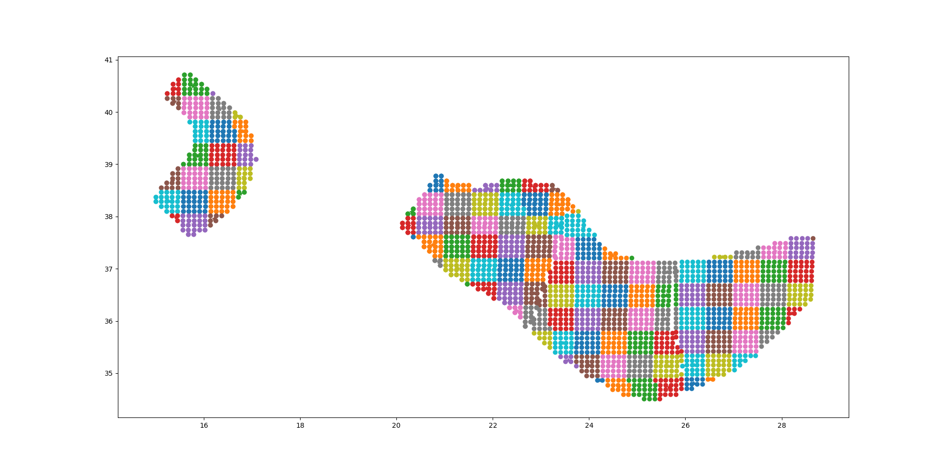
For distant sites it is possible to use the large grid (i.e. the CollapsePointSources) without losing much precision, while for close points the original sources must be used.
The engine uses the parameter pointsource_distance
to determine when to use the original sources and when to use the
collapsed sources.
If the maximum_distance has a value of 500 km and the
pointsource_distance a value of 50 km, then (50/500)^2 = 1%
of the sites will be close and 99% of the sites will be far.
Therefore you will able to use the collapsed sources for
99% percent of the sites and a huge speedup is to big expected
(in reality things are a bit more complicated, since the engine also consider
the fact that ruptures have a finite size, but you get the idea).
16.1. Application: making the Canada model 26x faster#
In order to give a concrete example, I ran the Canada 2015 model on 7 cities
by using the following site_model.csv file:
custom_site_id |
lon |
lat |
vs30 |
z1pt0 |
z2pt5 |
montre |
-73 |
45 |
368 |
393.6006 |
1.391181 |
calgar |
-114 |
51 |
451 |
290.6857 |
1.102391 |
ottawa |
-75 |
45 |
246 |
492.3983 |
2.205382 |
edmont |
-113 |
53 |
372 |
389.0669 |
1.374081 |
toront |
-79 |
43 |
291 |
465.5151 |
1.819785 |
winnip |
-97 |
50 |
229 |
499.7842 |
2.393656 |
vancou |
-123 |
49 |
600 |
125.8340 |
0.795259 |
Notice that we are using a custom_site_id field to identify the cities.
This is possible only in engine versions >= 3.13, where custom_site_id
has been extended to accept strings of at most 6 characters, while
before only integers were accepted (we could have used a zip code instead).
If no special approximations are used, the calculation is extremely
slow, since the model is extremely large. On the the GEM cluster (320
cores) it takes over 2 hours to process the 7 cities. The dominating
operation, as of engine 3.13, is “computing mean_std” which takes, in
total, 925,777 seconds split across the 320 cores, i.e. around 48
minutes per core. This is way too much and it would make impossible to
run the full model with ~138,000 sites. An analysis shows that the
calculation time is totally dominated by the point sources. Moreover,
the engine prints a warning saying that I should use the
pointsource_distance approximation. Let’s do so, i.e. let us set
pointsource_distance = 50
in the job.ini file. That alone triples the speed of the engine, and the calculation times in “computing mean_std” goes down to 324,241 seconds, i.e. 16 minutes per core, in average. An analysis of the hazard curves shows that there is practically no difference between the original curves and the ones computed with the approximation on:
$ oq compare hcurves PGA <first_calc_id> <second_calc_id>
There are no differences within the tolerances atol=0.001, rtol=0%, sids=[0 1 2 3 4 5 6]
However, this is not enough. We are still too slow to run the full model in a reasonable amount of time. Enters the point source gridding. By setting
ps_grid_spacing=50
we can spectacularly reduce the calculation time to 35,974s, down by
nearly an order of magnitude! This time oq compare hcurves
produces some differences on the last city but they are minor and not
affecting the hazard maps:
$ oq compare hmaps PGA <first_calc_id> <third_calc_id>
There are no differences within the tolerances atol=0.001, rtol=0%, sids=[0 1 2 3 4 5 6]
The following table collects the results:
operation |
calc_time |
approx |
speedup |
computing mean_std |
925_777 |
no approx |
1x |
computing mean_std |
324_241 |
pointsource_distance |
3x |
computing mean_std |
35_974 |
ps_grid_spacing |
26x |
It should be noticed that if you have 130,000 sites it is likely that
there will be a few sites where the point source gridding
approximation gives results quite different for the exact results.
The commands oq compare allows you to figure out which are the
problematic sites, where they are and how big is the difference from
the exact results.
You should take into account that even the “exact” results have uncertainties due to all kind of reasons, so even a large difference can be quite acceptable. In particular if the hazard is very low you can ignore any difference since it will have no impact on the risk.
Points with low hazard are expected to have large differences, this is
why by default oq compare use an absolute tolerance of 0.001g, but
you can raise that to 0.01g or more. You can also give a relative
tolerance of 10% or more. Internally oq compare calls the
function numpy.allclose see
https://numpy.org/doc/stable/reference/generated/numpy.allclose.html
for a description of how the tolerances work.
By increasing the pointsource_distance parameter and decreasing the
ps_grid_spacing parameter one can make the approximation as
precise as wanted, at the expense of a larger runtime.
NB: the fact that the Canada model with 7 cities can be made 26 times
faster does not mean that the same speedup apply when you consider the full
130,000+ sites. A test with ps_grid_spacing=pointsource_distance=50
gives a speedup of 7 times, which is still very significant.
16.2. How to determine the “right” value for the ps_grid_spacing parameter#
The trick is to run a sensitivity analysis on a reduced calculation. Set in the job.ini something like this:
sensitivity_analysis = {'ps_grid_spacing': [0, 20, 40, 60]}
and then run:
$ OQ_SAMPLE_SITES=.01 oq engine --run job.ini
This will run sequentially 4 calculations with different values of the
ps_grid_spacing. The first calculation, the one with
ps_grid_spacing=0, is the exact calculation, with the approximation
disabled, to be used as reference.
Notice that setting the environment variable OQ_SAMPLE_SITES=.01
will reduced by 100x the number of sites: this is essential in order to
make the calculation times acceptable in large calculations.
After running the 4 calculations you can compare the times by using
oq show performance and the precision by using oq
compare. From that you can determine which value of the
ps_grid_spacing gives a good speedup with a decent
precision. Calculations with plenty of nodal planes and hypocenters
will benefit from lower values of ps_grid_spacing while
calculations with a single nodal plane and hypocenter for each source
will benefit from higher values of ps_grid_spacing.
If you are interested only in speed and not in precision, you can set
calculation_mode=preclassical, run the sensitivity analysis in parallel
very quickly and then use the ps_grid_spacing value corresponding to
the minimum weight of the source model, which can be read from the
logs. Here is the trick to run the calculations in parallel:
$ oq engine --multi --run job.ini -p calculation_mode=preclassical
And here is how to extract the weight information, in the example of Alaska, with job IDs in the range 31692-31695:
$ oq db get_weight 31692
<Row(description=Alaska{'ps_grid_spacing': 0}, message=tot_weight=1_929_504, max_weight=120_594, num_sources=150_254)>
$ oq db get_weight 31693
<Row(description=Alaska{'ps_grid_spacing': 20}, message=tot_weight=143_748, max_weight=8_984, num_sources=22_727)>
$ oq db get_weight 31694
<Row(description=Alaska{'ps_grid_spacing': 40}, message=tot_weight=142_564, max_weight=8_910, num_sources=6_245)>
$ oq db get_weight 31695
<Row(description=Alaska{'ps_grid_spacing': 60}, message=tot_weight=211_542, max_weight=13_221, num_sources=3_103)>
The lowest weight is 142_564, corresponding to a ps_grid_spacing
of 40km; since the weight is 13.5 times smaller than the weight for
the full calculation (1_929_504), this is the maximum speedup that we
can expect from using the approximation.
Note 1: the weighting algorithm changes at every release, so only relative weights at a fixed release are meaningful and it does not make sense to compare weights across engine releases.
Note 2: the precision and performance of the ps_grid_spacing approximation
change at every release: you should not expect to get the same numbers and
performance across releases even if the model is the same and the parameters
are the same.
17. disagg_by_src#
Given a system of various sources affecting a specific site,
one very common question to ask is: what are the more relevant sources,
i.e. which sources contribute the most to the mean hazard curve?
The engine is able to answer such question by setting the disagg_by_src
flag in the job.ini file. When doing that, the engine saves in
the datastore a 5-dimensional array called disagg_by_src with
dimensions (site ID, realization ID, intensity measure type,
intensity measure level, source ID). For that it is possible to extract
the contribution of each source to the mean hazard curve (interested
people should look at the code in the function check_disagg_by_src).
The array disagg_by_src can also be read as a pandas DataFrame,
then getting something like the following:
>> dstore.read_df('disagg_by_src', index='src_id')
               site_id  rlz_id  imt  lvl         value
ASCTRAS407           0       0  PGA    0  9.703749e-02
IF-CFS-GRID03        0       0  PGA    0  3.720510e-02
ASCTRAS407           0       0  PGA    1  6.735009e-02
IF-CFS-GRID03        0       0  PGA    1  2.851081e-02
ASCTRAS407           0       0  PGA    2  4.546237e-02
...                ...     ...  ...  ...           ...
IF-CFS-GRID03        0      31  PGA   17  6.830692e-05
ASCTRAS407           0      31  PGA   18  1.072884e-06
IF-CFS-GRID03        0      31  PGA   18  1.275539e-05
ASCTRAS407           0      31  PGA   19  1.192093e-07
IF-CFS-GRID03        0      31  PGA   19  5.960464e-07
The value field here is the probability of exceedence in the hazard
curve. The lvl field is an integer corresponding to the intensity
measure level in the hazard curve.
There is a consistency check comparing the mean hazard curves with the value obtained by composing the probabilities in the disagg_by_src` array, for the heighest level of each intensity measure type.
It should be noticed that many hazard models contain thousands of
sources and as a consequence the disagg_by_src matrix can be
impossible to compute without running out of memory. Even if you have
enough memory, having a very large disagg_by_src matrix is a bad
idea, so there is a limit on the size of the matrix, hard-coded to 4
GB. The way to circumvent the limit is to reduce the number of
sources: for instance you could convert point sources in multipoint
sources.
In engine 3.15 we also introduced the so-called “colon convention” on source
IDs: if you have many sources that for some reason should be collected
together - for instance because they all account for seismicity in the same
tectonic region, or because they are components of a same source but are split
into separate sources by magnitude - you
can tell the engine to collect them into one source in the disagg_by_src
matrix. The trick is to use IDs with the same prefix, a colon, and then a
numeric index. For instance, if you had 3 sources with IDs src_mag_6.65,
src_mag_6.75, src_mag_6.85, fragments of the same source with
different magnitudes, you could change their IDs to something like
src:0, src:1, src:2 and that would reduce the size of the
matrix disagg_by_src by 3 times by collecting together the contributions
of each source. There is no restriction on the numeric indices to start
from 0, so using the names src:665, src:675, src:685 would
work too and would be clearer: the IDs should be unique, however.
If the IDs are not unique and the engine determines that the underlying
sources are different, then an extension “semicolon + incremental index”
is automatically added. This is useful when the hazard modeler wants
to define a model where the more than one version of the same source appears
in one source model, having changed some of the parameters, or when varied
versions of a source appear in each branch of a logic tree. In that case,
the modeler should use always the exact same ID (i.e. without the colon and
numeric index): the engine will automatically distinguish the
sources during the calculation of the hazard curves and consider them the same
when saving the array disagg_by_src: you can see an example in the
test qa_tests_data/classical/case_79 in the engine code base. In that
case the source_info dataset will list 6 sources
ASCTRAS407;0, ASCTRAS407;1, ASCTRAS407;2, ASCTRAS407;3,
IF-CFS-GRID03;0, IF-CFS-GRID03;1 but the matrix disagg_by_src
will see only two sources ASCTRAS407 and IF-CFS-GRID03 obtained
by composing together the versions of the underlying sources.
In version 3.15 disagg_by_src was extended to work with mutually
exclusive sources, i.e. for the Japan model. You can see an example in
the test qa_tests_data/classical/case_27. However, the case of
mutually exclusive ruptures - an example is the New Madrid cluster
in the USA model - is not supported yet.
In some cases it is tricky to discern whether use of the colon convention or identical source IDs is appropriate. The following list indicates several possible cases that a user may encounter, and the appropriate approach to assigning source IDs. Note that this list includes the cases that have been tested so far, and is not a comprehensive list of all cases that may arise.
Sources in the same source group/source model are scaled alternatives of each other. For example, this occurs when for a given source, epistemic uncertainties such as occurrence rates or geometries are considered, but the modeller has pre-scaled the rates rather than including the alternative hypothesis in separate logic tree branches.
Naming approach: identical IDs.
Sources in different files are alternatives of each other, e.g. each is used in a different branch of the source model logic tree.
Naming approach: identical IDs.
A source is defined in OQ by numerous sources, either in the same file or different ones. For example, one could have a set of non-parametric sources, each with many rutpures, that are grouped together into single files by magnitude. Or, one could have many point sources that together represent the seismicity from one source.
Naming approach: colon convention
One source consists of many mutually exclusive sources, as in
qa_tests_data/classical/case_27.Naming approach: colon convention
Cases 1 and 2 could include include more than one source typology, as in
qa_tests_data/classical/case_79.
NB: disagg_by_src can be set to true only if the
ps_grid_spacing approximation is disabled. The reason is that the
ps_grid_spacing approximation builds effective sources which are
not in the original source model, thus breaking the connection between
the values of the matrix and the original sources.
18. The conditional spectrum calculator#
The conditional_spectrum calculator is an experimental calculator
introduced in version 3.13, which is able to compute the conditional
spectrum in the sense of Baker.
In order to perform a conditional spectrum calculation you need to specify (on top of the usual parameter of a classical calculation):
a reference intensity measure type (i.e.
imt_ref = SA(0.2))a cross correlation model (i.e.
cross_correlation = BakerJayaram2008)a set of poes (i.e.
poes = 0.01 0.1)
The engine will compute a mean conditional spectrum for each poe and site,
as well as the usual mean uniform hazard spectra. The following restrictions
are enforced:
the IMTs can only be of type
SAandPGAthe source model cannot contain mutually exclusive sources (i.e. you cannot compute the conditional spectrum for the Japan model)
An example can be found in the engine repository, in the directory openquake/qa_tests_data/conditional_spectrum/case_1. If you run it, you will get something like the following:
$ oq engine --run job.ini
...
 id | name
261 | Full Report
262 | Hazard Curves
260 | Mean Conditional Spectra
263 | Realizations
264 | Uniform Hazard Spectra
Exporting the output 260 will produce two files conditional-spectrum-0.csv
and conditional-spectrum-1.csv; the first will refer to the first poe,
the second to the second poe. Each file will have a structure like
the following:
 #,,,,"generated_by='OpenQuake engine 3.13.0-gitd78d717e66', start_date='2021-10-13T06:15:20', checksum=3067457643, imls=[0.99999, 0.61470], site_id=0, lon=0.0, lat=0.0"
sa_period,val0,std0,val1,std1
0.00000E+00,1.02252E+00,2.73570E-01,7.53388E-01,2.71038E-01
1.00000E-01,1.99455E+00,3.94498E-01,1.50339E+00,3.91337E-01
2.00000E-01,2.71828E+00,9.37914E-09,1.84910E+00,9.28588E-09
3.00000E-01,1.76504E+00,3.31646E-01,1.21929E+00,3.28540E-01
1.00000E+00,3.08985E-01,5.89767E-01,2.36533E-01,5.86448E-01
The number of columns will depend from the number of sites. The
conditional spectrum calculator, like the disaggregation calculator,
is mean to be run on a very small number of sites, normally one.
In this example there are two sites 0 and 1 and the columns val0
and val give the value of the conditional spectrum on such sites
respectively, while the columns std0 and std1 give the corresponding
standard deviations.
Conditional spectra for individual realizations are also computed and stored for debugging purposes, but they are not exportable.
The implementation was adapted from the paper Conditional Spectrum Computation Incorporating Multiple Causal Earthquakes and Ground-Motion Prediction Models by Ting Lin, Stephen C. Harmsen, Jack W. Baker, and Nicolas Luco (http://citeseerx.ist.psu.edu/viewdoc/download?doi=10.1.1.845.163&rep=rep1&type=pdf) and it is rather sophisticated. The core formula is implemented in the method openquake.hazardlib.contexts.get_cs_contrib.
The conditional_spectrum calculator, like the disaggregation calculator,
is a kind of post-calculator, i.e. you can run a regular classical calculation
and then compute the conditional_spectrum in post-processing by using
the --hc option.