3. Risk#
3.1. Introduction to the Risk Module#
The seismic risk results are calculated using the OpenQuake risk library, an open-source suite of tools for seismic risk assessment and loss estimation. This library is written in the Python programming language and available in the form of a “developers” release at the following location: gem/oq-engine.
The risk component of the OpenQuake engine can compute both scenario-based and probabilistic seismic damage and risk using various approaches. The following types of analysis are currently supported:
Scenario Damage Assessment, for the calculation of damage distribution statistics for a portfolio of buildings from a single earthquake rupture scenario taking into account aleatory and epistemic ground-motion variability.
Scenario Risk Assessment, for the calculation of individual asset and portfolio loss statistics due to a single earthquake rupture scenario taking into account aleatory and epistemic ground-motion variability. Correlation in the vulnerability of different assets of the same typology can also be taken into consideration.
Classical Probabilistic Seismic Damage Analysis, for the calculation of damage state probabilities over a specified time period, and probabilistic collapse maps, starting from the hazard curves computed following the classical integration procedure ((Cornell 1968), McGuire (1976)) as formulated by (Field, Jordan, and Cornell 2003).
Classical Probabilistic Seismic Risk Analysis, for the calculation of loss curves and loss maps, starting from the hazard curves computed following the classical integration procedure ((Cornell 1968), McGuire (1976)) as formulated by (Field, Jordan, and Cornell 2003).
Stochastic Event Based Probabilistic Seismic Damage Analysis, for the calculation of event damage tables starting from stochastic event sets. Other results such as damage-state-exceedance curves, probabilistic damage maps, and average annual damages or collapses can be obtained by post-processing the event damage tables.
Stochastic Event Based Probabilistic Seismic Risk Analysis, for the calculation of event loss tables starting from stochastic event sets. Other results such as loss-exceedance curves, probabilistic loss maps, and average annual losses can be obtained by post-processing the event loss tables.
Retrofit Benefit-Cost Ratio Analysis, which is useful in estimating the net-present value of the potential benefits of performing retrofitting for a portfolio of assets (in terms of decreased losses in seismic events), measured relative to the upfront cost of retrofitting.
Each calculation workflow has a modular structure, so that intermediate results can be saved and analyzed. Moreover, each calculator can be extended independently of the others so that additional calculation options and methodologies can be easily introduced, without affecting the overall calculation workflow. Each workflow is described in more detail in the following sections.
3.1.1. Scenario Damage Assessment#
The scenario damage calculator computes damage distribution statistics for all assets in a given Exposure Model for a single specified rupture. Damage distribution statistics include the mean and standard deviation of damage fractions for different damage states. This calculator requires the definition of a finite Rupture Model, an Exposure Model and a Fragility Model; the main results are the damage distribution statistics per asset, aggregated damage distribution statistics per taxonomy, aggregated damage distribution statistics for the region, and collapse maps, which contain the spatial distribution of the number or area of collapsed buildings throughout the region of interest.
The rupture characteristics—i.e. the magnitude, hypocenter and fault geometry—are modelled as deterministic in the scenario calculators. Multiple simulations of different possible Ground Motion Fields due to the single rupture are generated, taking into consideration both the inter-event variability of ground motions, and the intra-event residuals obtained from a spatial correlation model for ground motion residuals. The use of logic trees allows for the consideration of uncertainty in the choice of a ground motion model for the given tectonic region.
As an alternative to computing the Ground Motion Fields with OpenQuake engine, users can also provide their own sets of Ground Motion Fields as input to the scenario damage calculator.
Note: The damage simulation algorithm for the scenario damage calculator has changed starting from OpenQuake engine39 to use a full Monte Carlo simulation of damage states.
For each Ground Motion Field, a damage state is simulated for each building for every asset in the Exposure Model using the provided Fragility Model, and finally the mean damage distribution across all realizations is calculated. The calculator also provides aggregated damage distribution statistics for the portfolio, such as mean damage fractions for each taxonomy in the Exposure Model, and the mean damage for the entire region of study.
The required input files required for running a scenario damage calculation and the resulting output files are depicted in Fig. 3.1.
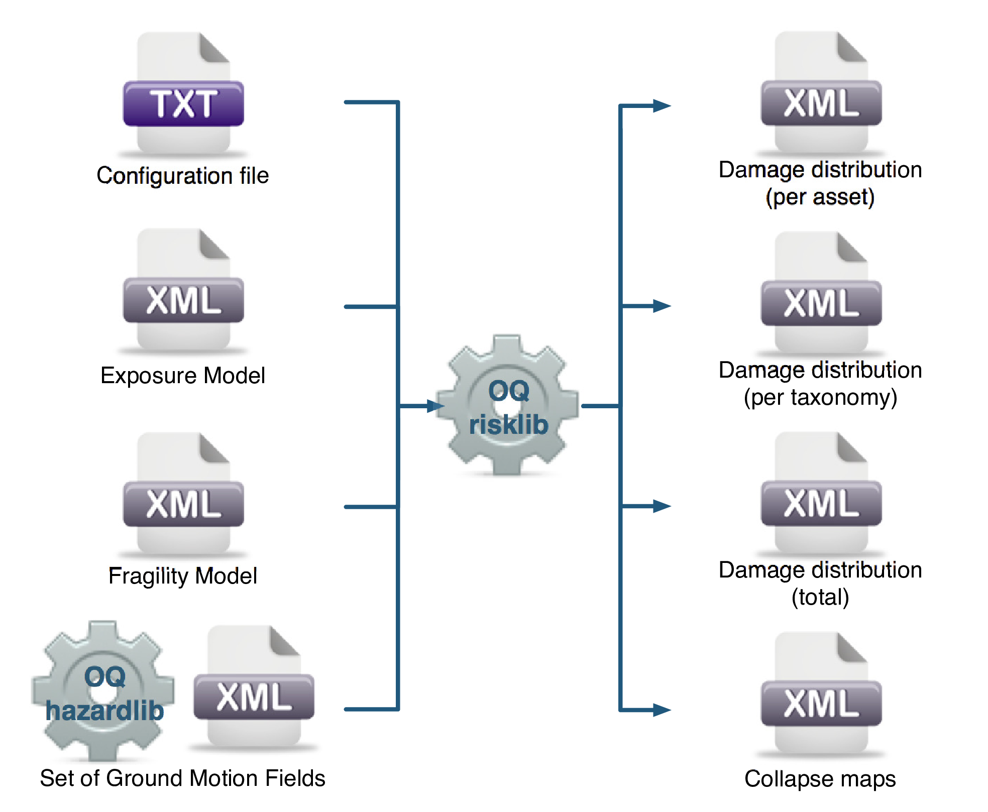
Fig. 3.1 Scenario Damage Calculator input/output structure.#
Consequence Model files can also be provided as inputs for a scenario damage calculation in addition to fragilitymodels files, in order to estimate consequences based on the calculated damage distribution. The user may provide one Consequence Model file corresponding to each loss type (amongst structural, nonstructural, contents, and business interruption) for which a Fragility Model file is provided. Whereas providing a Fragility Model file for at least one loss type is mandatory for running a Scenario Damage calculation, providing corresponding Consequence Model files is optional.
3.1.2. Scenario Risk Assessment#
The scenario risk calculator computes loss statistics for all assets in a given Exposure Model for a single specified rupture. Loss statistics include the mean and standard deviation of ground-up losses for each loss type considered in the analysis. Loss statistics can currently be computed for five different loss types using this calculator: structural losses, nonstructural losses, contents losses, downtime losses, and occupant fatalities. This calculator requires the definition of a finite Rupture Model, an Exposure Model and a Vulnerability Model for each loss type considered; the main results are the loss statistics per asset and mean loss maps.
The rupture characteristics—i.e. the magnitude, hypocenter and fault geometry—are modelled as deterministic in the scenario calculators. Multiple simulations of different possible Ground Motion Fields due to the single rupture are generated, taking into consideration both the inter-event variability of ground motions, and the intra-event residuals obtained from a spatial correlation model for ground motion residuals. The use of logic trees allows for the consideration of uncertainty in the choice of a ground motion model for the given tectonic region.
As an alternative to computing the Ground Motion Fields with OpenQuake, users can also provide their own sets of Ground Motion Fields as input to the scenario risk calculator.
For each Ground Motion Field simulation, a loss ratio is sampled for every asset in the Exposure Model using the provided probabilistic Vulnerability Model taking into consideration the correlation model for vulnerability of different assets of a given taxonomy. Finally loss statistics, i.e., the mean loss and standard deviation of loss for ground-up losses across all simulations, are calculated for each asset. Mean loss maps are also generated by this calculator, describing the mean ground-up losses caused by the scenario event for the different assets in the Exposure Model.
The required input files required for running a scenario risk calculation and the resulting output files are depicted in Fig. 3.2.
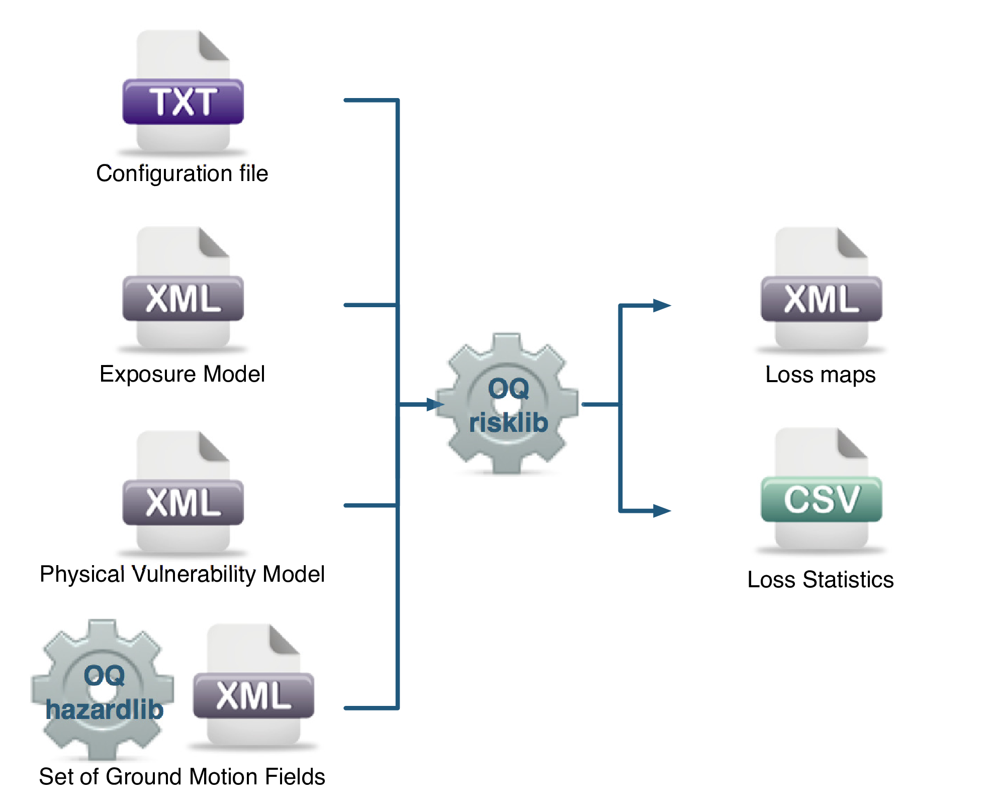
Fig. 3.2 Scenario Risk Calculator input/output structure.#
3.1.3. Classical Probabilistic Seismic Damage Analysis#
The classical PSHA-based damage calculator integrates the fragility functions for an asset with the seismic hazard curve at the location of the asset, to give the expected damage distribution for the asset within a specified time period. The calculator requires the definition of an Exposure Model, a Fragility Model with fragilityfunctions for each taxonomy represented in the Exposure Model, and hazard curves calculated in the region of interest. The main results of this calculator are the expected damage distribution for each asset, which describe the probability of the asset being in different damage states, and collapse maps for the region, which describe the probability of collapse for different assets in the portfolio over the specified time period. Damage distribution aggregated by taxonomy or of the total portfolio (considering all assets in the Exposure Model) can not be extracted using this calculator, as the spatial correlation of the ground motion residuals is not taken into consideration.
The hazard curves required for this calculator can be calculated by the OpenQuake engine for all asset locations in the Exposure Model using the classical PSHA approach (Cornell 1968; McGuire 1976).
The required input files required for running a classical probabilistic damage calculation and the resulting output files are depicted in Fig. 3.3.
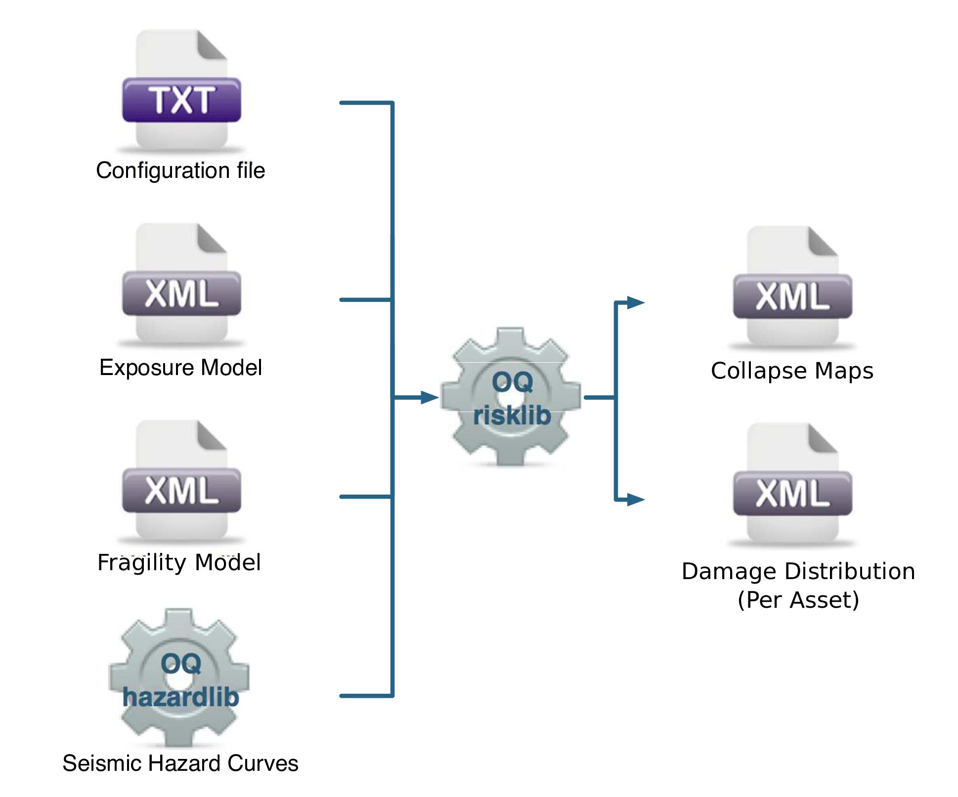
Fig. 3.3 Classical PSHA-based Damage Calculator input/output structure.#
3.1.4. Classical Probabilistic Seismic Risk Analysis#
The classical PSHA-based risk calculator convolves through numerical integration, the probabilistic vulnerability functions for an asset with the seismic hazard curve at the location of the asset, to give the loss distribution for the asset within a specified time period. The calculator requires the definition of an Exposure Model, a Vulnerability Model for each loss type of interest with vulnerabilityfunctions for each taxonomy represented in the Exposure Model, and hazard curves calculated in the region of interest. Loss curves and loss maps can currently be calculated for five different loss types using this calculator: structural losses, nonstructural losses, contents losses, downtime losses, and occupant fatalities. The main results of this calculator are loss exceedance curves for each asset, which describe the probability of exceedance of different loss levels over the specified time period, and loss maps for the region, which describe the loss values that have a given probability of exceedance over the specified time
Unlike the probabilistic event-based risk calculator, an aggregate loss curve (considering all assets in the Exposure Model) can not be extracted using this calculator, as the correlation of the ground motion residuals and vulnerability uncertainty is not taken into consideration in this calculator.
The hazard curves required for this calculator can be calculated by the OpenQuake engine for all asset locations in the Exposure Model using the classical PSHA approach (Cornell 1968; McGuire 1976). The use of logic- trees allows for the consideration of model uncertainty in the choice of a ground motion prediction equation for the different tectonic region types in the region. Unlike what was described in the previous calculator, a total loss curve (considering all assets in the Exposure Model) can not be extracted using this calculator, as the correlation of the ground motion residuals and vulnerability uncertainty is not taken into consideration.
The required input files required for running a classical probabilistic risk calculation and the resulting output files are depicted in Fig. 3.4.
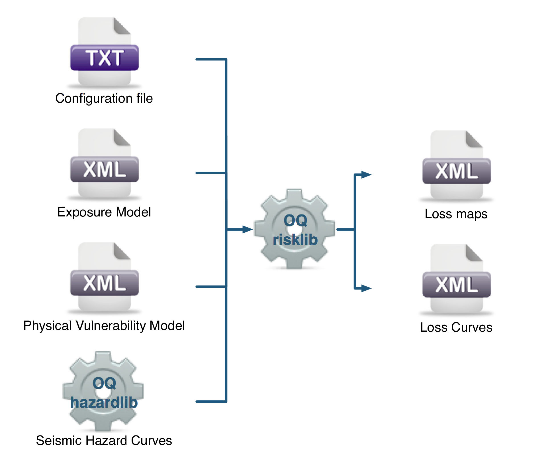
Fig. 3.4 Classical PSHA-based Risk Calculator input/output structure.#
3.1.5. Stochastic Event Based Probabilistic Seismic#
Damage Analysis This calculator employs an event-based Monte Carlo simulation approach to probabilistic damage assessment in order to estimate the damage distribution for individual assets and aggregated damage distribution for a spatially distributed portfolio of assets within a specified time period. The calculator requires the definition of an Exposure Model, a Fragility Model for each loss type of interest with fragilityfunctions for each damage state for every typology represented in the Exposure Model, and a Stochastic Event Set representative of the seismicity of the region over the specified time period. Damage state curves and damage maps corresponding to specified return periods can also be obtained using this calculator.
As an alternative to computing the Ground Motion Fields with OpenQuake engine, users can also provide their own sets of Ground Motion Fields as input to the event-based damage calculator.
The main results of this calculator are the event damage tables; these tables describe the total number of buildings in each damage state for the portfolio of assets for each seismic event in the Stochastic Event Set.
Asset-level event damage tables are generated by the calculator, but are not exportable in csv format due to the large file sizes that may be involved. Interested users can access the asset-level event damage tables within the datastore for the completed calculation.
This calculator relies on the probabilistic event-based hazard calculator, which simulates the seismicity of the chosen time period \(T\) by producing a Stochastic Event Set. For each rupture generated by a Seismic Source, the number of occurrences in the given time span \(T\) is simulated by sampling the corresponding probability distribution as given by \(P_{rup}(k | T)\). A Stochastic Event Set is therefore a sample of the full population of ruptures as defined by a Seismic Source Model. Each rupture is present zero, one or more times, depending on its probability. Symbolically, we can define a Stochastic Event Set as:
where \(k\), the number of occurrences, is a random sample of \(P_{rup}(k | T)\), and \(k \times rup\) means that rupture \(rup\) is repeated \(k\) times in the Stochastic Event Set.
For each rupture or event in the Stochastic Event Sets, a spatially correlated Ground Motion Field realisation is generated, taking into consideration both the inter-event variability of ground motions, and the intra-event residuals obtained from a spatial correlation model for ground motion residuals (if one is specified in the job file). The use of logic trees allows for the consideration of uncertainty in the choice of a Seismic Source Model, and in the choice of groundmotionmodels for the different tectonic regions.
For each Ground Motion Field realization, a damage state is siumulated for each building of every asset in the Exposure Model using the provided Fragility Model. The asset-level event damage table is saved to the datastore. Time-averaged damage distributions at the asset-level can be obtained from the event damage table. Finally damage state exceedance curves can be computed.
The required input files required for running a probabilistic stochastic event-based damage calculation and the resulting output files are depicted in Fig. 3.5.
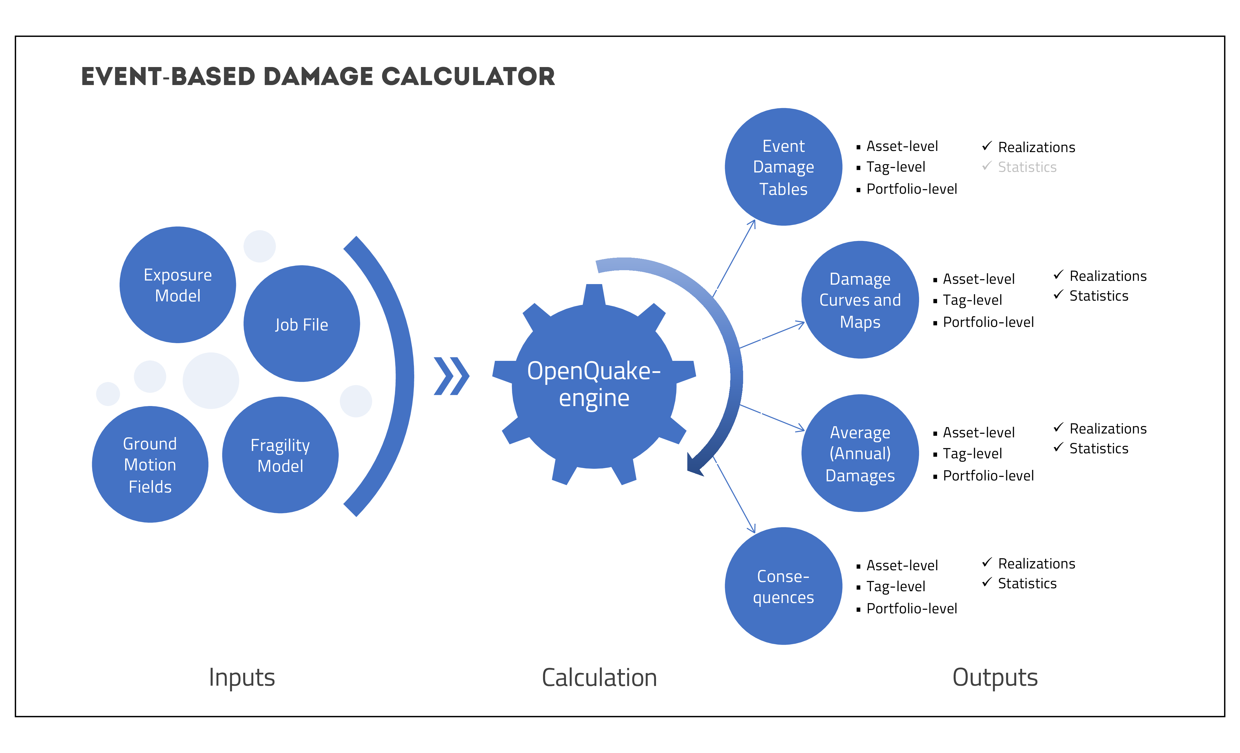
Fig. 3.5 Probabilistic Event-based Damage Calculator input/output structure.#
Similar to the scenario damage calculator, Consequence Model files can also be provided as inputs for an event-based damage calculation in addition to fragilitymodels files, in order to estimate consequences based on the calculated damage distribution. The user may provide one Consequence Model file corresponding to each loss type (amongst structural, nonstructural, contents, and business interruption) for which a Fragility Model file is provided. Whereas providing a Fragility Model file for at least one loss type is mandatory for running an Event-Based Damage calculation, providing corresponding Consequence Model files is optional.
3.1.6. Stochastic Event Based Probabilistic Seismic#
Risk Analysis This calculator employs an event-based Monte Carlo simulation approach to probabilistic risk assessment in order to estimate the loss distribution for individual assets and aggregated loss distribution for a spatially distributed portfolio of assets within a specified time period. The calculator requires the definition of an Exposure Model, a Vulnerability Model for each loss type of interest with vulnerabilityfunctions for each taxonomy represented in the Exposure Model, and a Stochastic Event Set (also known as a synthetic catalog) representative of the seismicity of the region over the specified time period. Loss curves and loss maps can currently be calculated for five different loss types using this calculator: structural losses, nonstructural losses, contents losses, downtime losses, and occupant fatalities.
As an alternative to computing the Ground Motion Fields with OpenQuake engine, users can also provide their own sets of Ground Motion Fields as input to the event-based risk calculator, starting from OpenQuake engine28.
The main results of this calculator are loss exceedance curves for each asset, which describe the probability of exceedance of different loss levels over the specified time period, and loss maps for the region, which describe the loss values that have a given probability of exceedance over the specified time period. Aggregate loss exceedance curves can also be produced using this calculator; these describe the probability of exceedance of different loss levels for all assets in the portfolio. Finally, event loss tables can be produced using this calculator; these tables describe the total loss across the portfolio for each seismic event in the Stochastic Event Set.
This calculator relies on the probabilistic event-based hazard calculator, which simulates the seismicity of the chosen time period \(T\) by producing a Stochastic Event Set. For each rupture generated by a Seismic Source, the number of occurrences in the given time span \(T\) is simulated by sampling the corresponding probability distribution as given by \(P_{rup}(k | T)\). A Stochastic Event Set is therefore a sample of the full population of ruptures as defined by a Seismic Source Model. Each rupture is present zero, one or more times, depending on its probability. Symbolically, we can define a Stochastic Event Set as:
where \(k\), the number of occurrences, is a random sample of \(P_{rup}(k | T)\), and \(k \times rup\) means that rupture \(rup\) is repeated \(k\) times in the Stochastic Event Set.
For each rupture or event in the Stochastic Event Sets, a spatially correlated Ground Motion Field realisation is generated, taking into consideration both the inter-event variability of ground motions, and the intra-event residuals obtained from a spatial correlation model for ground motion residuals (if one is specified in the job file). The use of logic trees allows for the consideration of uncertainty in the choice of a Seismic Source Model, and in the choice of groundmotionmodels for the different tectonic regions.
For each Ground Motion Field realization, a loss ratio is sampled for every asset in the Exposure Model using the provided probabilistic Vulnerability Model, taking into consideration the correlation model for vulnerability of different assets of a given taxonomy. Finally loss exceedance curves are computed for ground-up losses.
The required input files required for running a probabilistic stochastic event-based risk calculation and the resulting output files are depicted in Fig. 3.6.
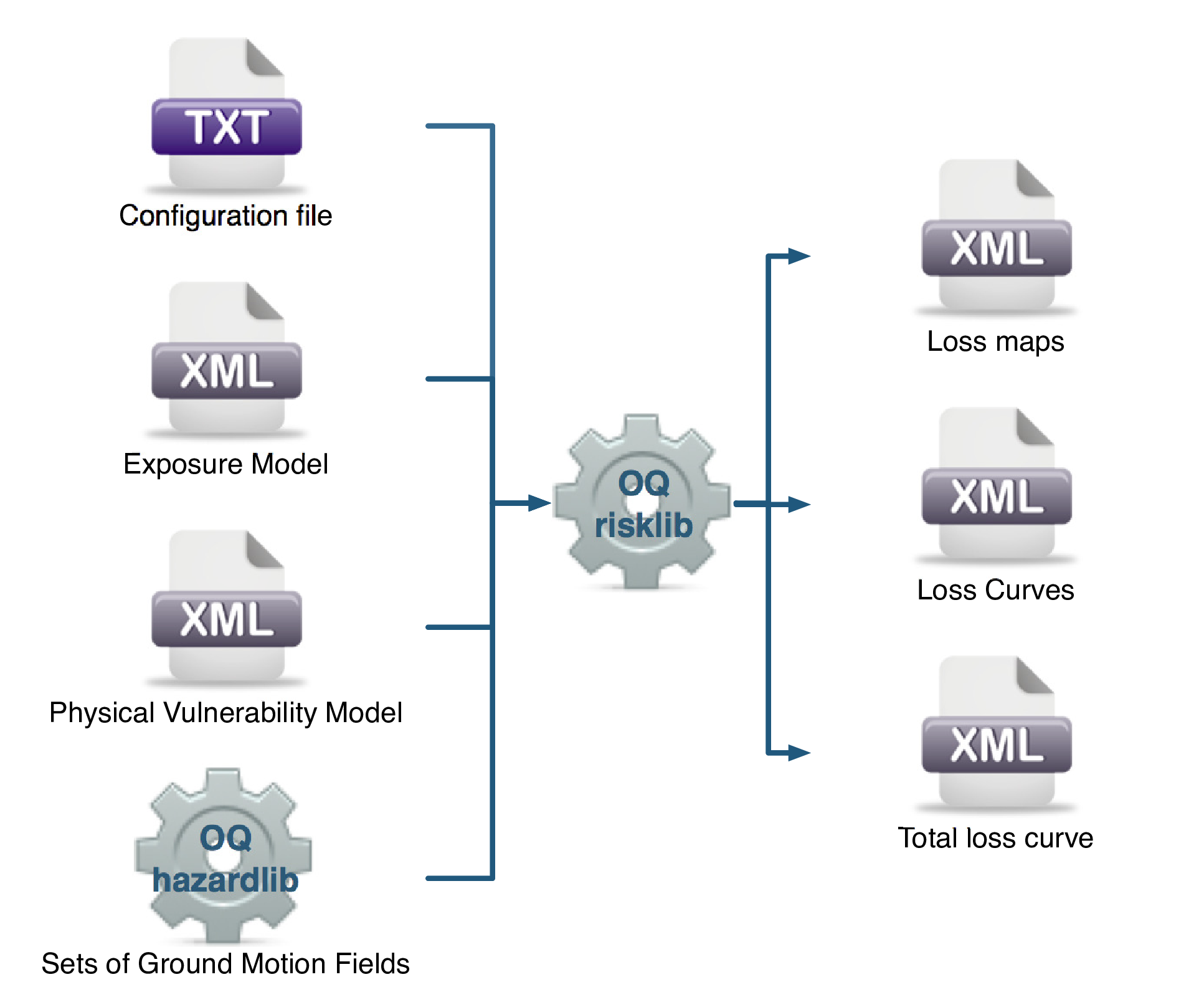
Fig. 3.6 Probabilistic Event-based Risk Calculator input/output structure.#
3.1.7. Retrofit Benefit-Cost Ratio Analysis#
This calculator represents a decision-support tool for deciding whether the employment of retrofitting measures to a collection of existing buildings is advantageous from an economical point of view. For this assessment, the expected losses considering the original and retrofitted configuration of the buildings are estimated, and the economic benefit due to the better seismic design is divided by the retrofitting cost, leading to the benefit/cost ratio. These loss curves are computed using the previously described Classical PSHA- based Risk calculator. The output of this calculator is a benefit/cost ratio for each asset, in which a ratio above one indicates that employing a retrofitting intervention is economically viable.
In Fig. 3.7, the input/output structure for this calculator is depicted.
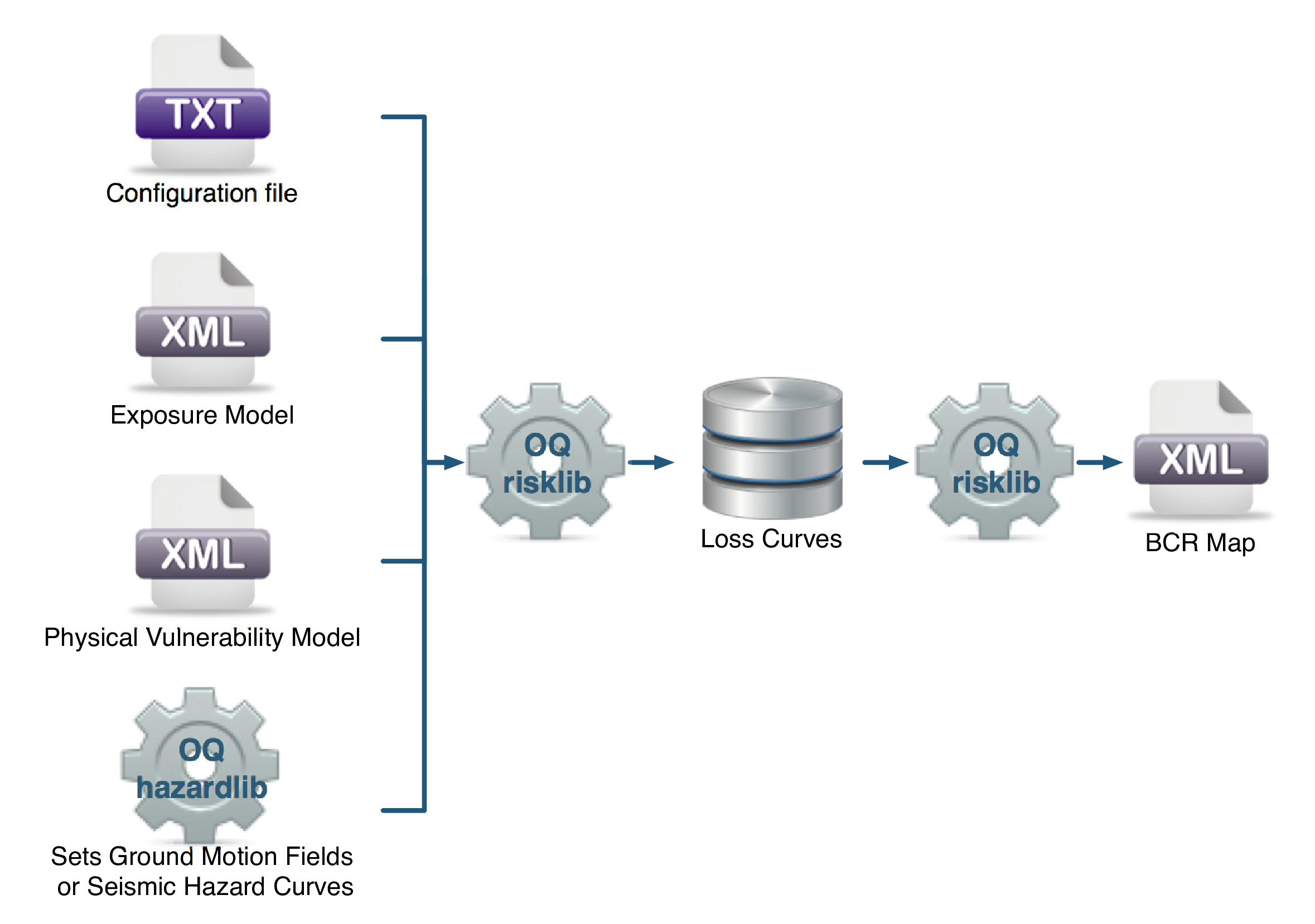
Fig. 3.7 Retrofitting Benefit/Cost Ratio Calculator input/output structure.#
For further information regarding the theoretical background of the methodologies used for each calculator, users are referred to the OpenQuake- engine Book (Risk).
3.2. Risk Input Models#
The following sections describe the basic inputs required for a risk calculation, including exposuremodels, fragilitymodels, consequencemodels, and vulnerabilitymodels. In addition, each risk calculator also requires the appropriate hazard inputs computed in the region of interest. Hazard inputs include hazard curves for the classical probabilistic damage and risk calculators, Ground Motion Field for the scenario damage and risk calculators, or Stochastic Event Sets for the probabilistic event based calculators.
3.2.1. Exposure Models#
All risk calculators in the OpenQuake engine require an Exposure Model that needs to be provided in the Natural hazards’ Risk Markup Language schema, the use of which is illustrated through several examples in this section. The information included in an Exposure Model comprises a metadata section listing general information about the exposure, followed by a cost conversions section that describes how the different areas, costs, and occupancies for the assets will be specified, followed by data regarding each individual asset in the portfolio.
Note: Starting from OpenQuake engine30, the Exposure Model may be provided using csv files listing the asset information, along with an xml file conatining the metadata section for the exposure model that has been described in the examples above. See Example 8 below for an illustration of an exposure model using csv files.
A simple Exposure Model comprising a single asset is shown in the listing below.
 1<?xml version="1.0" encoding="UTF-8"?>
 2<nrml xmlns:gml="http://www.opengis.net/gml"
 3      xmlns="http://openquake.org/xmlns/nrml/0.5">
 4
 5<exposureModel id="exposure_example"
 6               category="buildings"
 7               taxonomySource="GEM_Building_Taxonomy_2.0">
 8  <description>Exposure Model Example</description>
 9
10  <conversions>
11    <costTypes>
12      <costType name="structural" type="per_area" unit="USD" />
13    </costTypes>
14    <area type="per_asset" unit="SQM" />
15  </conversions>
16
17  <assets>
18    <asset id="a1" taxonomy="Adobe" number="5" area="100" >
19      <location lon="-122.000" lat="38.113" />
20      <costs>
21        <cost type="structural" value="10000" />
22      </costs>
23      <occupancies>
24        <occupancy occupants="20" period="day" />
25      </occupancies>
26    </asset>
27  </assets>
28
29</exposureModel>
30
31</nrml>
Let us take a look at each of the sections in the above example file in turn. The first part of the file contains the metadata section:
 1<?xml version="1.0" encoding="UTF-8"?>
 2<nrml xmlns:gml="http://www.opengis.net/gml"
 3      xmlns="http://openquake.org/xmlns/nrml/0.5">
 4
 5<exposureModel id="exposure_example"
 6               category="buildings"
 7               taxonomySource="GEM_Building_Taxonomy_2.0">
 8  <description>Exposure Model Example</description>
 9
10  <conversions>
11    <costTypes>
12      <costType name="structural" type="per_area" unit="USD" />
13    </costTypes>
14    <area type="per_asset" unit="SQM" />
15  </conversions>
16
17  <assets>
18    <asset id="a1" taxonomy="Adobe" number="5" area="100" >
19      <location lon="-122.000" lat="38.113" />
20      <costs>
21        <cost type="structural" value="10000" />
22      </costs>
23      <occupancies>
24        <occupancy occupants="20" period="day" />
25      </occupancies>
26    </asset>
27  </assets>
28
29</exposureModel>
30
31</nrml>
The information in the metadata section is common to all of the assets in the portfolio and needs to be incorporated at the beginning of every Exposure Model file. There are a number of parameters that compose the metadata section, which is intended to provide general information regarding the assets within the Exposure Model. These parameters are described below:
id: mandatory; a unique string used to identify the Exposure Model. This string can contain letters (a–z; A–Z), numbers (0–9), dashes (–), and underscores (_), with a maximum of 100 characters.category: an optional string used to define the type of assets being stored (e.g: buildings, lifelines).taxonomySource: an optional attribute used to define the taxonomy being used to classify the assets.description: mandatory; a brief string (ASCII) with further information about the Exposure Model.
Next, let us look at the part of the file describing the area and cost conversions:
 1<?xml version="1.0" encoding="UTF-8"?>
 2<nrml xmlns:gml="http://www.opengis.net/gml"
 3      xmlns="http://openquake.org/xmlns/nrml/0.5">
 4
 5<exposureModel id="exposure_example"
 6               category="buildings"
 7               taxonomySource="GEM_Building_Taxonomy_2.0">
 8  <description>Exposure Model Example</description>
 9
10  <conversions>
11    <costTypes>
12      <costType name="structural" type="per_area" unit="USD" />
13    </costTypes>
14    <area type="per_asset" unit="SQM" />
15  </conversions>
16
17  <assets>
18    <asset id="a1" taxonomy="Adobe" number="5" area="100" >
19      <location lon="-122.000" lat="38.113" />
20      <costs>
21        <cost type="structural" value="10000" />
22      </costs>
23      <occupancies>
24        <occupancy occupants="20" period="day" />
25      </occupancies>
26    </asset>
27  </assets>
28
29</exposureModel>
30
31</nrml>
Notice that the costType element defines a name, a type, and
a unit attribute.
The Natural hazards’ Risk Markup Language schema for the Exposure Model allows the definition of a
structural cost, a nonstructural components cost, a contents cost, and a
business interruption or downtime cost for each asset in the portfolio.
Thus, the valid values for the name attribute of the costType
element are the following:
structural: used to specify the structural replacement cost of assetsnonstructural: used to specify the replacement cost for the nonstructural components of assetscontents: used to specify the contents replacement costbusiness_interruption: used to specify the cost that will be incurred per unit time that a damaged asset remains closed following an earthquake
The Exposure Model shown in the example above defines only the structural values for the assets. However, multiple cost types can be defined for each asset in the same Exposure Model.
The unit attribute of the costType element is used for
specifying the currency unit for the corresponding cost type. Note that
the OpenQuake engine itself is agnostic to the currency units; the unit is
thus a descriptive attribute which is used by the OpenQuake engine to annotate
the results of a risk assessment. This attribute can be set to any valid
Unicode string.
The type attribute of the costType element specifies whether the
costs will be provided as an aggregated value for an asset, or per
building or unit comprising an asset, or per unit area of an asset. The
valid values for the type attribute of the costType element are
the following:
aggregated: indicates that the replacement costs will be provided as an aggregated value for each assetper_asset: indicates that the replacement costs will be provided per structural unit comprising each assetper_area: indicates that the replacement costs will be provided per unit area for each asset
If the costs are to be specified per_area for any of the
costTypes, the area element will also need to be defined in the
conversions section. The area element defines a type, and a
unit attribute.
The unit attribute of the area element is used for specifying
the units for the area of an asset. The OpenQuake engine itself is agnostic to
the area units; the unit is thus a descriptive attribute which is
used by the OpenQuake engine to annotate the results of a risk assessment. This
attribute can be set to any valid ASCII string.
The type attribute of the area element specifies whether the
area will be provided as an aggregated value for an asset, or per
building or unit comprising an asset. The valid values for the type
attribute of the area element are the following:
aggregated: indicates that the area will be provided as an aggregated value for each assetper_asset: indicates that the area will be provided per building or unit comprising each asset
The way the information about the characteristics of the assets in an Exposure Model are stored can vary strongly depending on how and why the data was compiled. As an example, if national census information is used to estimated the distribution of assets in a given region, it is likely that the number of buildings within a given geographical area will be used to define the dataset, and will be used for estimating the number of collapsed buildings for a scenario earthquake. On the other hand, if simplified methodologies based on proxy data such as population distribution are used to develop the Exposure Model, then it is likely that the built up area or economic cost of each building typology will be directly derived, and will be used for the estimation of economic losses.
Finally, let us look at the part of the file describing the set of assets in the portfolio to be used in seismic damage or risk calculations:
 1<?xml version="1.0" encoding="UTF-8"?>
 2<nrml xmlns:gml="http://www.opengis.net/gml"
 3      xmlns="http://openquake.org/xmlns/nrml/0.5">
 4
 5<exposureModel id="exposure_example"
 6               category="buildings"
 7               taxonomySource="GEM_Building_Taxonomy_2.0">
 8  <description>Exposure Model Example</description>
 9
10  <conversions>
11    <costTypes>
12      <costType name="structural" type="per_area" unit="USD" />
13    </costTypes>
14    <area type="per_asset" unit="SQM" />
15  </conversions>
16
17  <assets>
18    <asset id="a1" taxonomy="Adobe" number="5" area="100" >
19      <location lon="-122.000" lat="38.113" />
20      <costs>
21        <cost type="structural" value="10000" />
22      </costs>
23      <occupancies>
24        <occupancy occupants="20" period="day" />
25      </occupancies>
26    </asset>
27  </assets>
28
29</exposureModel>
30
31</nrml>
Each asset definition involves specifiying a set of mandatory and optional attributes concerning the asset. The following set of attributes can be assigned to each asset based on the current schema for the Exposure Model:
id: mandatory; a unique string used to identify the given asset, which is used by the OpenQuake engine to relate each asset with its associated results. This string can contain letters (a–z; A–Z), numbers (0–9), dashes (-), and underscores (_), with a maximum of 100 characters.taxonomy: mandatory; this string specifies the building typology of the given asset. The taxonomy strings can be user-defined, or based on an existing classification scheme such as the GEM Taxonomy, PAGER, or EMS-98.number: the number of individual structural units comprising a given asset. This attribute is mandatory for damage calculations. For risk calculations, this attribute must be defined if either the area or any of the costs are provided per structural unit comprising each asset.area: area of the asset, at a given location. As mentioned earlier, the area is a mandatory attribute only if any one of the costs for the asset is specified per unit area.location: mandatory; specifies the longitude (between -180\(^{\circ}\) to 180\(^{\circ}\)) and latitude (between -90\(^{\circ}\) to 90 \(^{\circ}\)) of the given asset, both specified in decimal degrees 2.costs: specifies a set of costs for the given asset. The replacement value for different cost types must be provided on separate lines within thecostselement. As shown in the example above, each cost entry must define thetypeand thevalue. Currently supported valid options for the costtypeare:structural,nonstructural,contents, andbusiness_interruption.occupancies: mandatory only for probabilistic or scenario risk calculations that specify anoccupants_vulnerability_file. Each entry within this element specifies the number of occupants for the asset for a particular period of the day. As shown in the example above, each occupancy entry must define theperiodand theoccupants. Currently supported valid options for theperiodare:day,transit, andnight. Currently, the number ofoccupantsfor an asset can only be provided as an aggregated value for the asset.
For the purposes of performing a retrofitting benefit/cost analysis, it
is also necessary to define the retrofitting cost (retrofitted). The
combination between the possible options in which these three attributes
can be defined leads to four ways of storing the information about the
assets. For each of these cases a brief explanation and example is
provided in this section.
Example 1
This example illustrates an Exposure Model in which the aggregated cost (structural, nonstructural, contents and business interruption) of the assets of each taxonomy for a set of locations is directly provided. Thus, in order to indicate how the various costs will be defined, the following information needs to be stored in the Exposure Model file, as shown in the listing below.
 1<?xml version="1.0" encoding="UTF-8"?>
 2<nrml xmlns:gml="http://www.opengis.net/gml"
 3      xmlns="http://openquake.org/xmlns/nrml/0.5">
 4
 5<exposureModel id="exposure_example"
 6               category="buildings"
 7               taxonomySource="GEM_Building_Taxonomy_2.0">
 8  <description>
 9    Exposure model with aggregated replacement costs for each asset
10  </description>
11  <conversions>
12    <costTypes>
13      <costType name="structural" type="aggregated" unit="USD" />
14      <costType name="nonstructural" type="aggregated" unit="USD" />
15      <costType name="contents" type="aggregated" unit="USD" />
16      <costType name="business_interruption" type="aggregated" unit="USD/month"/>
17    </costTypes>
18  </conversions>
19  <assets>
20    <asset id="a1" taxonomy="Adobe" >
21      <location lon="-122.000" lat="38.113" />
22      <costs>
23        <cost type="structural" value="20000" />
24        <cost type="nonstructural" value="30000" />
25        <cost type="contents" value="10000" />
26        <cost type="business_interruption" value="4000" />
27      </costs>
28    </asset>
29  </assets>
30</exposureModel>
31
32</nrml>
In this case, the cost type of each component as been defined as
aggregated. Once the way in which each cost is going to be defined
has been established, the values for each asset can be stored according
to the format shown in
the listing.
 1<?xml version="1.0" encoding="UTF-8"?>
 2<nrml xmlns:gml="http://www.opengis.net/gml"
 3      xmlns="http://openquake.org/xmlns/nrml/0.5">
 4
 5<exposureModel id="exposure_example"
 6               category="buildings"
 7               taxonomySource="GEM_Building_Taxonomy_2.0">
 8  <description>
 9    Exposure model with aggregated replacement costs for each asset
10  </description>
11  <conversions>
12    <costTypes>
13      <costType name="structural" type="aggregated" unit="USD" />
14      <costType name="nonstructural" type="aggregated" unit="USD" />
15      <costType name="contents" type="aggregated" unit="USD" />
16      <costType name="business_interruption" type="aggregated" unit="USD/month"/>
17    </costTypes>
18  </conversions>
19  <assets>
20    <asset id="a1" taxonomy="Adobe" >
21      <location lon="-122.000" lat="38.113" />
22      <costs>
23        <cost type="structural" value="20000" />
24        <cost type="nonstructural" value="30000" />
25        <cost type="contents" value="10000" />
26        <cost type="business_interruption" value="4000" />
27      </costs>
28    </asset>
29  </assets>
30</exposureModel>
31
32</nrml>
Each asset is uniquely identified by its id. Then, a pair of
coordinates (latitude and longitude) for a location where the asset
is assumed to exist is defined. Each asset must be classified according
to a taxonomy, so that the OpenQuake engine is capable of employing the
appropriate Vulnerability Function or Fragility Function in the risk
calculations. Finally, the cost values of each type are stored
within the costs attribute. In this example, the aggregated value
for all structural units (within a given asset) at each location is
provided directly, so there is no need to define other attributes such
as number or area. This mode of representing an Exposure Model is
probably the simplest one.
Example 2
In the snippet shown in the listing below, an Exposure Model containing the number of structural units and the associated costs per unit of each asset is presented.
 1<?xml version="1.0" encoding="UTF-8"?>
 2<nrml xmlns:gml="http://www.opengis.net/gml"
 3      xmlns="http://openquake.org/xmlns/nrml/0.5">
 4
 5<exposureModel id="exposure_example"
 6               category="buildings"
 7               taxonomySource="GEM_Building_Taxonomy_2.0">
 8  <description>
 9    Exposure model with replacement costs per building for each asset
10  </description>
11  <conversions>
12    <costTypes>
13      <costType name="structural" type="per_asset" unit="USD" />
14      <costType name="nonstructural" type="per_asset" unit="USD" />
15      <costType name="contents" type="per_asset" unit="USD" />
16      <costType name="business_interruption" type="per_asset" unit="USD/month"/>
17    </costTypes>
18  </conversions>
19  <assets>
20    <asset id="a1" number="2" taxonomy="Adobe" >
21      <location lon="-122.000" lat="38.113" />
22      <costs>
23        <cost type="structural" value="7500" />
24        <cost type="nonstructural" value="11250" />
25        <cost type="contents" value="3750" />
26        <cost type="business_interruption" value="1500" />
27      </costs>
28    </asset>
29  </assets>
30</exposureModel>
31
32</nrml>
For this case, the cost type has been set to per_asset. Then,
the information from each asset can be stored following the format shown
in
the listing below.
 1<?xml version="1.0" encoding="UTF-8"?>
 2<nrml xmlns:gml="http://www.opengis.net/gml"
 3      xmlns="http://openquake.org/xmlns/nrml/0.5">
 4
 5<exposureModel id="exposure_example"
 6               category="buildings"
 7               taxonomySource="GEM_Building_Taxonomy_2.0">
 8  <description>
 9    Exposure model with replacement costs per building for each asset
10  </description>
11  <conversions>
12    <costTypes>
13      <costType name="structural" type="per_asset" unit="USD" />
14      <costType name="nonstructural" type="per_asset" unit="USD" />
15      <costType name="contents" type="per_asset" unit="USD" />
16      <costType name="business_interruption" type="per_asset" unit="USD/month"/>
17    </costTypes>
18  </conversions>
19  <assets>
20    <asset id="a1" number="2" taxonomy="Adobe" >
21      <location lon="-122.000" lat="38.113" />
22      <costs>
23        <cost type="structural" value="7500" />
24        <cost type="nonstructural" value="11250" />
25        <cost type="contents" value="3750" />
26        <cost type="business_interruption" value="1500" />
27      </costs>
28    </asset>
29  </assets>
30</exposureModel>
31
32</nrml>
In this example, the various costs for each asset is not provided
directly, as in the previous example. In order to carry out the risk
calculations in which the economic cost of each asset is provided, the
OpenQuake engine multiplies, for each asset, the number of units (buildings) by
the “per asset” replacement cost. Note that in this case, there is no
need to specify the attribute area.
Example 3
The example shown in the listing below comprises an Exposure Model containing the built up area of each asset, and the associated costs are provided per unit area.
 1<?xml version="1.0" encoding="UTF-8"?>
 2<nrml xmlns:gml="http://www.opengis.net/gml"
 3      xmlns="http://openquake.org/xmlns/nrml/0.5">
 4
 5<exposureModel id="exposure_example"
 6               category="buildings"
 7               taxonomySource="GEM_Building_Taxonomy_2.0">
 8  <description>
 9    Exposure model with replacement costs per unit area;
10    and areas provided as aggregated values for each asset
11  </description>
12  <conversions>
13    <area type="aggregated" unit="SQM" />
14    <costTypes>
15      <costType name="structural" type="per_area" unit="USD" />
16      <costType name="nonstructural" type="per_area" unit="USD" />
17      <costType name="contents" type="per_area" unit="USD" />
18      <costType name="business_interruption" type="per_area" unit="USD/month"/>
19    </costTypes>
20  </conversions>
21  <assets>
22    <asset id="a1" area="1000" taxonomy="Adobe" >
23      <location lon="-122.000" lat="38.113" />
24      <costs>
25        <cost type="structural" value="5" />
26        <cost type="nonstructural" value="7.5" />
27        <cost type="contents" value="2.5" />
28        <cost type="business_interruption" value="1" />
29      </costs>
30    </asset>
31  </assets>
32</exposureModel>
33
34</nrml>
In order to compile an Exposure Model with this structure, the cost
type should be set to per_area. In addition, it is also
necessary to specify if the area that is being store represents the
aggregated area of number of units within an asset, or the average area
of a single unit. In this particular case, the area that is being
stored is the aggregated built up area per asset, and thus this
attribute was set to aggregated.
The listing below
illustrates the definition of the assets for this example.
 1<?xml version="1.0" encoding="UTF-8"?>
 2<nrml xmlns:gml="http://www.opengis.net/gml"
 3      xmlns="http://openquake.org/xmlns/nrml/0.5">
 4
 5<exposureModel id="exposure_example"
 6               category="buildings"
 7               taxonomySource="GEM_Building_Taxonomy_2.0">
 8  <description>
 9    Exposure model with replacement costs per unit area;
10    and areas provided as aggregated values for each asset
11  </description>
12  <conversions>
13    <area type="aggregated" unit="SQM" />
14    <costTypes>
15      <costType name="structural" type="per_area" unit="USD" />
16      <costType name="nonstructural" type="per_area" unit="USD" />
17      <costType name="contents" type="per_area" unit="USD" />
18      <costType name="business_interruption" type="per_area" unit="USD/month"/>
19    </costTypes>
20  </conversions>
21  <assets>
22    <asset id="a1" area="1000" taxonomy="Adobe" >
23      <location lon="-122.000" lat="38.113" />
24      <costs>
25        <cost type="structural" value="5" />
26        <cost type="nonstructural" value="7.5" />
27        <cost type="contents" value="2.5" />
28        <cost type="business_interruption" value="1" />
29      </costs>
30    </asset>
31  </assets>
32</exposureModel>
33
34</nrml>
Once again, the OpenQuake engine needs to carry out some calculations in order to
compute the different costs per asset. In this case, this value is
computed by multiplying the aggregated built up area of each asset
by the associated cost per unit area. Notice that in this case, there is
no need to specify the attribute number.
Example 4
This example demonstrates an Exposure Model that defines the number of structural units for each asset, the average built up area per structural unit and the associated costs per unit area. The listing below shows the metadata definition for an Exposure Model built in this manner.
 1<?xml version="1.0" encoding="UTF-8"?>
 2<nrml xmlns:gml="http://www.opengis.net/gml"
 3      xmlns="http://openquake.org/xmlns/nrml/0.5">
 4
 5<exposureModel id="exposure_example"
 6               category="buildings"
 7               taxonomySource="GEM_Building_Taxonomy_2.0">
 8  <description>
 9    Exposure model with replacement costs per unit area;
10    and areas provided per building for each asset
11  </description>
12  <conversions>
13    <area type="per_asset" unit="SQM" />
14    <costTypes>
15      <costType name="structural" type="per_area" unit="USD" />
16      <costType name="nonstructural" type="per_area" unit="USD" />
17      <costType name="contents" type="per_area" unit="USD" />
18      <costType name="business_interruption" type="per_area" unit="USD/month"/>
19    </costTypes>
20  </conversions>
21  <assets>
22    <asset id="a1" number="3" area="400" taxonomy="Adobe" >
23      <location lon="-122.000" lat="38.113" />
24      <costs>
25        <cost type="structural" value="10" />
26        <cost type="nonstructural" value="15" />
27        <cost type="contents" value="5" />
28        <cost type="business_interruption" value="2" />
29      </costs>
30    </asset>
31  </assets>
32</exposureModel>
33
34</nrml>
Similarly to what was described in the previous example, the various
costs type also need to be established as per_area, but the
type of area is now defined as per_asset.
The listing below
illustrates the definition of the assets for this example.
 1<?xml version="1.0" encoding="UTF-8"?>
 2<nrml xmlns:gml="http://www.opengis.net/gml"
 3      xmlns="http://openquake.org/xmlns/nrml/0.5">
 4
 5<exposureModel id="exposure_example"
 6               category="buildings"
 7               taxonomySource="GEM_Building_Taxonomy_2.0">
 8  <description>
 9    Exposure model with replacement costs per unit area;
10    and areas provided per building for each asset
11  </description>
12  <conversions>
13    <area type="per_asset" unit="SQM" />
14    <costTypes>
15      <costType name="structural" type="per_area" unit="USD" />
16      <costType name="nonstructural" type="per_area" unit="USD" />
17      <costType name="contents" type="per_area" unit="USD" />
18      <costType name="business_interruption" type="per_area" unit="USD/month"/>
19    </costTypes>
20  </conversions>
21  <assets>
22    <asset id="a1" number="3" area="400" taxonomy="Adobe" >
23      <location lon="-122.000" lat="38.113" />
24      <costs>
25        <cost type="structural" value="10" />
26        <cost type="nonstructural" value="15" />
27        <cost type="contents" value="5" />
28        <cost type="business_interruption" value="2" />
29      </costs>
30    </asset>
31  </assets>
32</exposureModel>
33
34</nrml>
In this example, the OpenQuake engine will make use of all the parameters to estimate the various costs of each asset, by multiplying the number of structural units by its average built up area, and then by the respective cost per unit area.
Example 5
In this example, additional information will be included, which is required for other risk analysis besides loss estimation, such as the benefit/cost analysis.
In order to perform a benefit/cost assessment, it is necessary to indicate the retrofitting cost. This parameter is handled in the same manner as the structural cost, and it should be stored according to the format shown in the listing below.
 1<?xml version="1.0" encoding="UTF-8"?>
 2<nrml xmlns:gml="http://www.opengis.net/gml"
 3      xmlns="http://openquake.org/xmlns/nrml/0.5">
 4
 5<exposureModel id="exposure_example"
 6               category="buildings"
 7               taxonomySource="GEM_Building_Taxonomy_2.0">
 8  <description>Exposure model illustrating retrofit costs</description>
 9  <conversions>
10    <costTypes>
11      <costType name="structural" type="aggregated" unit="USD"
12                retrofittedType="per_asset" retrofittedUnit="USD" />
13    </costTypes>
14  </conversions>
15  <assets>
16    <asset id="a1" taxonomy="Adobe" number="1" >
17      <location lon="-122.000" lat="38.113" />
18      <costs>
19        <cost type="structural" value="10000" retrofitted="2000" />
20      </costs>
21    </asset>
22  </assets>
23</exposureModel>
24
25</nrml>
Despite the fact that for the demonstration of how the retrofitting cost can be stored the per building type of cost structure described in Example 1 was used, it is important to mention that any of the other cost storing approaches can also be employed (Examples 2–4).
Example 6
The OpenQuake engine is also capable of estimating human losses, based on the number of occupants in an asset, at a certain time of the day. The example Exposure Model shown in the listing below illustrates how this parameter is defined for each asset. In addition, this example also serves the purpose of presenting an Exposure Model in which three cost types have been defined using three different options.
As previously mentioned, in this example only three costs are being
stored, and each one follows a different approach. The structural
cost is being defined as the aggregate replacement cost for all of the
buildings comprising the asset (Example 1), the nonstructural value
is defined as the replacement cost per unit area where the area is
defined per building comprising the asset (Example 4), and the
contents and business_interruption values are provided per
building comprising the asset (Example 2). The number of occupants at
different times of the day are also provided as aggregated values for
all of the buildings comprising the asset.
 1<?xml version="1.0" encoding="UTF-8"?>
 2<nrml xmlns:gml="http://www.opengis.net/gml"
 3      xmlns="http://openquake.org/xmlns/nrml/0.5">
 4
 5<exposureModel id="exposure_example"
 6               category="buildings"
 7               taxonomySource="GEM_Building_Taxonomy_2.0">
 8  <description>Exposure model example with occupants</description>
 9  <conversions>
10    <costTypes>
11      <costType name="structural" type="aggregated" unit="USD" />
12      <costType name="nonstructural" type="per_area" unit="USD" />
13      <costType name="contents" type="per_asset" unit="USD" />
14      <costType name="business_interruption" type="per_asset" unit="USD/month" />
15    </costTypes>
16    <area type="per_asset" unit="SQM" />
17  </conversions>
18  <assets>
19    <asset id="a1" taxonomy="Adobe" number="5" area="200" >
20      <location lon="-122.000" lat="38.113" />
21      <costs>
22        <cost type="structural" value="20000" />
23        <cost type="nonstructural" value="15" />
24        <cost type="contents" value="2400" />
25        <cost type="business_interruption" value="1500" />
26      </costs>
27      <occupancies>
28        <occupancy occupants="6" period="day" />
29        <occupancy occupants="10" period="transit" />
30        <occupancy occupants="20" period="night" />
31      </occupancies>
32    </asset>
33  </assets>
34</exposureModel>
35
36</nrml>
Example 7
Starting from OpenQuake engine27, the user may also provide a set of tags for each asset in the Exposure Model. The primary intended use case for the tags is to enable aggregation or accumulation of risk results (casualties / damages / losses) for each tag. The tags could be used to specify location attributes, occupancy types, or insurance policy codes for the different assets in the Exposure Model.
The example Exposure Model shown in the listing below illustrates how one or more tags can be defined for each asset.
 1<?xml version="1.0" encoding="UTF-8"?>
 2<nrml xmlns:gml="http://www.opengis.net/gml"
 3      xmlns="http://openquake.org/xmlns/nrml/0.5">
 4
 5<exposureModel id="exposure_example_with_tags"
 6               category="buildings"
 7               taxonomySource="GEM_Building_Taxonomy_2.0">
 8  <description>Exposure Model Example with Tags</description>
 9
10  <conversions>
11    <costTypes>
12      <costType name="structural" type="per_area" unit="USD" />
13    </costTypes>
14    <area type="per_asset" unit="SQM" />
15  </conversions>
16
17  <tagNames>state county tract city zip cresta</tagNames>
18
19  <assets>
20    <asset id="a1" taxonomy="Adobe" number="5" area="100" >
21      <location lon="-122.000" lat="38.113" />
22      <costs>
23        <cost type="structural" value="10000" />
24      </costs>
25      <occupancies>
26        <occupancy occupants="20" period="day" />
27      </occupancies>
28      <tags state="California" county="Solano" tract="252702"
29            city="Suisun" zip="94585" cresta="A.11"/>
30    </asset>
31  </assets>
32
33</exposureModel>
34
35</nrml>
The list of tag names that will be used in the Exposure Model must be provided in the metadata section of the exposure file, as shown in the following snippet from the full file:
 1<?xml version="1.0" encoding="UTF-8"?>
 2<nrml xmlns:gml="http://www.opengis.net/gml"
 3      xmlns="http://openquake.org/xmlns/nrml/0.5">
 4
 5<exposureModel id="exposure_example_with_tags"
 6               category="buildings"
 7               taxonomySource="GEM_Building_Taxonomy_2.0">
 8  <description>Exposure Model Example with Tags</description>
 9
10  <conversions>
11    <costTypes>
12      <costType name="structural" type="per_area" unit="USD" />
13    </costTypes>
14    <area type="per_asset" unit="SQM" />
15  </conversions>
16
17  <tagNames>state county tract city zip cresta</tagNames>
18
19  <assets>
20    <asset id="a1" taxonomy="Adobe" number="5" area="100" >
21      <location lon="-122.000" lat="38.113" />
22      <costs>
23        <cost type="structural" value="10000" />
24      </costs>
25      <occupancies>
26        <occupancy occupants="20" period="day" />
27      </occupancies>
28      <tags state="California" county="Solano" tract="252702"
29            city="Suisun" zip="94585" cresta="A.11"/>
30    </asset>
31  </assets>
32
33</exposureModel>
34
35</nrml>
The tag values for the different tags can then be specified for each asset as shown in the following snippet from the same file:
 1<?xml version="1.0" encoding="UTF-8"?>
 2<nrml xmlns:gml="http://www.opengis.net/gml"
 3      xmlns="http://openquake.org/xmlns/nrml/0.5">
 4
 5<exposureModel id="exposure_example_with_tags"
 6               category="buildings"
 7               taxonomySource="GEM_Building_Taxonomy_2.0">
 8  <description>Exposure Model Example with Tags</description>
 9
10  <conversions>
11    <costTypes>
12      <costType name="structural" type="per_area" unit="USD" />
13    </costTypes>
14    <area type="per_asset" unit="SQM" />
15  </conversions>
16
17  <tagNames>state county tract city zip cresta</tagNames>
18
19  <assets>
20    <asset id="a1" taxonomy="Adobe" number="5" area="100" >
21      <location lon="-122.000" lat="38.113" />
22      <costs>
23        <cost type="structural" value="10000" />
24      </costs>
25      <occupancies>
26        <occupancy occupants="20" period="day" />
27      </occupancies>
28      <tags state="California" county="Solano" tract="252702"
29            city="Suisun" zip="94585" cresta="A.11"/>
30    </asset>
31  </assets>
32
33</exposureModel>
34
35</nrml>
Note that it is not mandatory that every tag name specified in the metadata section must be provided with a tag value for each asset.
Example 8
This example illustrates the use of multiple csv files containing the assets information, in conjunction with the metadata section in the usual xml format.
Let us take a look at the metadata section of the Exposure Model, which is listed as usual in an xml file:
 1<?xml version="1.0" encoding="UTF-8"?>
 2<nrml xmlns:gml="http://www.opengis.net/gml"
 3      xmlns="http://openquake.org/xmlns/nrml/0.5">
 4
 5<exposureModel id="exposure_example_with_csv_files"
 6               category="buildings"
 7               taxonomySource="GEM_Building_Taxonomy_3.0">
 8  <description>Exposure Model Example with CSV Files</description>
 9
10  <conversions>
11    <costTypes>
12      <costType name="structural" type="aggregated" unit="USD" />
13      <costType name="nonstructural" type="aggregated" unit="USD" />
14      <costType name="contents" type="aggregated" unit="USD" />
15    </costTypes>
16    <area type="per_asset" unit="SQFT" />
17  </conversions>
18
19  <occupancyPeriods>night</occupancyPeriods>
20
21  <tagNames>occupancy state_id state county_id county tract</tagNames>
22
23  <assets>
24    Washington.csv
25    Oregon.csv
26    California.csv
27  </assets>
28
29</exposureModel>
30
31</nrml>
As in all previous examples, the information in the metadata section is common to all of the assets in the portfolio.
The asset data can be provided in one or more csv files. The path to
each of the csv files containing the asset data must be listed between
the <assets> and </assets> xml tags.
In the example shown above, the exposure information is provided in three csv files, Washington.csv, Oregon.csv, and California.csv. To illustrate the format of the csv files, we have shown below the header and first few lines of the file Washington.csv in Table 3.1.
id |
lon |
lat |
taxonomy |
number |
structural |
area |
occupancy |
state |
county |
|---|---|---|---|---|---|---|---|---|---|
A1 |
-122.7 |
46.5 |
AGR1-W1-LC |
7.6 |
898000 |
18 |
Agr |
Washington |
Lewis County |
A2 |
-122.7 |
46.5 |
AGR1-PC1-LC |
0.6 |
67000 |
1 |
Agr |
Washington |
Lewis County |
A3 |
-122.7 |
46.5 |
AGR1-C2L-PC |
0.6 |
67000 |
1 |
Agr |
Washington |
Lewis County |
A4 |
-122.7 |
46.5 |
AGR1-PC1-PC |
1.5 |
179000 |
4 |
Agr |
Washington |
Lewis County |
A5 |
-122.7 |
46.5 |
AGR1-S2L-LC |
0.6 |
67000 |
1 |
Agr |
Washington |
Lewis County |
A6 |
-122.7 |
46.5 |
AGR1-S1L-PC |
1.1 |
133000 |
3 |
Agr |
Washington |
Lewis County |
A7 |
-122.7 |
46.5 |
AGR1-S2L-PC |
1.5 |
182000 |
4 |
Agr |
Washington |
Lewis County |
A8 |
-122.7 |
46.5 |
AGR1-S3-PC |
1.1 |
133000 |
3 |
Agr |
Washington |
Lewis County |
A9 |
-122.7 |
46.5 |
AGR1-RM1L-LC |
0.6 |
68000 |
1 |
Agr |
Washington |
Lewis County |
Note that the xml metadata section for exposure models provided using
csv files must include the xml tag <occupancyPeriods> listing the
periods of day for which the number of occupants in each asset will be
listed in the csv files. In case the number of occupants are not listed
in the csv files, a self-closing tag <occupancyPeriods /> should be
included in the xml metadata section.
A web-based tool to build an Exposure Model in the Natural hazards’ Risk Markup Language schema starting from a csv file or a spreadsheet can be found at the OpenQuake platform at the following address: https://platform.openquake.org/ipt/.
3.2.2. Fragility Models#
This section describes the schema currently used to store fragilitymodels, which are required for the Scenario Damage Calculator and the Classical Probabilistic Seismic Damage Calculator. In order to perform probabilistic or scenario damage calculations, it is necessary to define a Fragility Function for each building typology present in the Exposure Model. A Fragility Model defines a set of fragilityfunctions, describing the probability of exceeding a set of limit, or damage, states. The fragilityfunctions can be defined using either a discrete or a continuous format, and the Fragility Model file can include a mix of both types of fragilityfunctions.
For discrete fragilityfunctions, sets of probabilities of exceedance (one set per limit state) are defined for a list of intensity measure levels, as illustrated in Fig. 3.8.

Fig. 3.8 Graphical representation of a discrete fragility model#
The fragilityfunctions can also be defined as continuous functions, through the use of cumulative lognormal distribution functions. In Fig. 3.9, a continuous Fragility Model is presented.
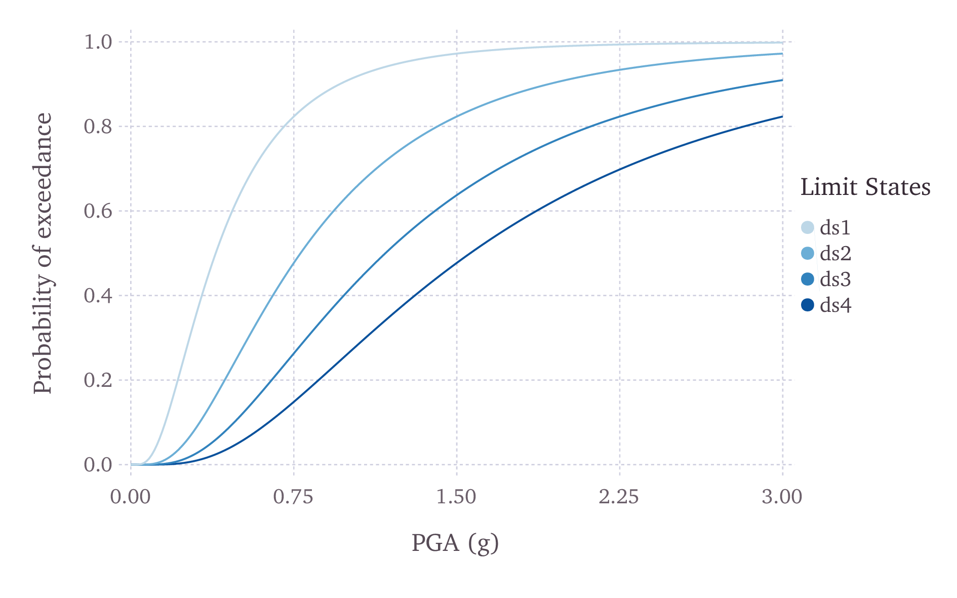
Fig. 3.9 Graphical representation of a continuous fragility model#
An example Fragility Model comprising one discrete Fragility Function and one continuous Fragility Function is shown in the listing below.
 1<?xml version="1.0" encoding="UTF-8"?>
 2<nrml xmlns="http://openquake.org/xmlns/nrml/0.5">
 3
 4<fragilityModel id="fragility_example"
 5                assetCategory="buildings"
 6                lossCategory="structural">
 7
 8  <description>Fragility Model Example</description>
 9  <limitStates>slight moderate extensive complete</limitStates>
10
11  <fragilityFunction id="Woodframe_TwoStorey" format="discrete">
12    <imls imt="PGA" noDamageLimit="0.05">0.005 0.2 0.4 0.6 0.8 1.0 1.2</imls>
13    <poes ls="slight">0.00 0.01 0.15 0.84 0.99 1.00 1.00</poes>
14    <poes ls="moderate">0.00 0.00 0.01 0.12 0.35 0.57 0.74</poes>
15    <poes ls="extensive">0.00 0.00 0.00 0.08 0.19 0.32 0.45</poes>
16    <poes ls="complete">0.00 0.00 0.00 0.06 0.17 0.26 0.35</poes>
17  </fragilityFunction>
18
19  <fragilityFunction id="RC_LowRise" format="continuous" shape="logncdf">
20    <imls imt="SA(0.3)" noDamageLimit="0.05" minIML="0.0" maxIML="5.0"/>
21    <params ls="slight" mean="0.50" stddev="0.10"/>
22    <params ls="moderate" mean="1.00" stddev="0.40"/>
23    <params ls="extensive" mean="1.50" stddev="0.90"/>
24    <params ls="complete" mean="2.00" stddev="1.60"/>
25  </fragilityFunction>
26
27</fragilityModel>
28
29</nrml>
The initial portion of the schema contains general information that describes some general aspects of the Fragility Model. The information in this metadata section is common to all of the functions in the Fragility Model and needs to be included at the beginning of every Fragility Model file. The parameters of the metadata section are shown in the snippet below and described after the snippet:
4<fragilityModel id="fragility_example"
5                assetCategory="buildings"
6                lossCategory="structural">
7
8  <description>Fragility Model Example</description>
9  <limitStates>slight moderate extensive complete</limitStates>
id: mandatory; a unique string used to identify the Fragility Model. This string can contain letters (a–z; A–Z), numbers (0–9), dashes (-), and underscores (_), with a maximum of 100 characters.assetCategory: an optional string used to specify the type of assets for which fragilityfunctions will be defined in this file (e.g: buildings, lifelines).lossCategory: mandatory; valid strings for this attribute are “structural”, “nonstructural”, “contents”, and “business_interruption”.description: mandatory; a brief string (ASCII) with further relevant information about the Fragility Model, for example, which building typologies are covered or the source of the functions in the Fragility Model.limitStates: mandatory; this field is used to define the number and nomenclature of each limit state. Four limit states are employed in the example above, but it is possible to use any number of discrete states, as long as a fragility curve is always defined for each limit state. The limit states must be provided as a set of strings separated by whitespaces between each limit state. Each limit state string can contain letters (a–z; A–Z), numbers (0–9), dashes (-), and underscores (_). Please ensure that there is no whitespace within the name of any individual limit state.
The following snippet from the above Fragility Model example file defines a discrete Fragility Function:
19  <fragilityFunction id="Woodframe_TwoStorey" format="discrete">
20    <imls imt="PGA" noDamageLimit="0.05">0.005 0.2 0.4 0.6 0.8 1.0 1.2</imls>
21    <poes ls="slight">0.00 0.01 0.15 0.84 0.99 1.00 1.00</poes>
22    <poes ls="moderate">0.00 0.00 0.01 0.12 0.35 0.57 0.74</poes>
23    <poes ls="extensive">0.00 0.00 0.00 0.08 0.19 0.32 0.45</poes>
24    <poes ls="complete">0.00 0.00 0.00 0.06 0.17 0.26 0.35</poes>
25  </fragilityFunction>
The following attributes are needed to define a discrete Fragility Function:
id: mandatory; a unique string used to identify the taxonomy for which the function is being defined. This string is used to relate the Fragility Function with the relevant asset in the Exposure Model. This string can contain letters (a–z; A–Z), numbers (0–9), dashes (-), and underscores (_), with a maximum of 100 characters.format: mandatory; for discrete fragilityfunctions, this attribute should be set to “discrete”.imls: mandatory; this attribute specifies the list of intensity levels for which the limit state probabilities of exceedance will be defined. In addition, it is also necessary to define the intensity measure type (imt). Optionally, anoDamageLimitcan be specified, which defines the intensity level below which the probability of exceedance for all limit states is taken to be zero.poes: mandatory; this field is used to define the probabilities of exceedance (poes) for each limit state for each discrete Fragility Function. It is also necessary to specify which limit state the exceedance probabilities are being defined for using the attributels. The probabilities of exceedance for each limit state must be provided on a separate line; and the number of exceedance probabilities for each limit state defined by thepoesattribute must be equal to the number of intensity levels defined by the attributeimls. Finally, the number and names of the limit states in each fragility function must be equal to the number of limit states defined earlier in the metadata section of the Fragility Model using the attributelimitStates.
The following snippet from the above Fragility Model example file defines a continuous Fragility Function:
11  <fragilityFunction id="RC_LowRise" format="continuous" shape="logncdf">
12    <imls imt="SA(0.3)" noDamageLimit="0.05" minIML="0.0" maxIML="5.0"/>
13    <params ls="slight" mean="0.50" stddev="0.10"/>
14    <params ls="moderate" mean="1.00" stddev="0.40"/>
15    <params ls="extensive" mean="1.50" stddev="0.90"/>
16    <params ls="complete" mean="2.00" stddev="1.60"/>
17  </fragilityFunction>
The following attributes are needed to define a continuous Fragility Function:
id: mandatory; a unique string used to identify the taxonomy for which the function is being defined. This string is used to relate the Fragility Function with the relevant asset in the Exposure Model. This string can contain letters (a–z; A–Z), numbers (0–9), dashes (-), and underscores (_), with a maximum of 100 characters.format: mandatory; for continuous fragilityfunctions, this attribute should be set to “continuous”.shape: mandatory; for continuous fragilityfunctions using the lognormal cumulative distrution, this attribute should be set to “logncdf”. At present, only the lognormal cumulative distribution function can be used for representing continuous fragilityfunctions.imls: mandatory; this element specifies aspects related to the intensity measure used by the the Fragility Function. The range of intensity levels for which the continuous fragilityfunctions are valid is specified using the attributesminIMLandmaxIML. In addition, it is also necessary to define the intensity measure typeimt. Optionally, anoDamageLimitcan be specified, which defines the intensity level below which the probability of exceedance for all limit states is taken to be zero.params: mandatory; this field is used to define the parameters of the continuous curve for each limit state for this Fragility Function. For a lognormal cumulative distrbution function, the two parameters required to specify the function are the mean and standard deviation of the intensity level. These parameters are defined for each limit state using the attributesmeanandstddevrespectively. The attributelsspecifies the limit state for which the parameters are being defined. The parameters for each limit state must be provided on a separate line. The number and names of the limit states in each Fragility Function must be equal to the number of limit states defined earlier in the metadata section of the Fragility Model using the attributelimitStates. A point worth clarifying is that the parameters to be defined in the fragility input file are the mean and standard deviation of the intensity measure level (IML) for each damage state, and not the mean and standard deviation of log(IML). Thus, if the intensity measure is PGA or SA for instance, the units for the input parameters will be ’g’.
Note that the schema for representing fragilitymodels has changed between Natural hazards’ Risk Markup Language v0.4 (used prior to OpenQuake engine17) and Natural hazards’ Risk Markup Language v0.5 (introduced in OpenQuake engine17).
A deprecation warning is printed every time you attempt to use a
Fragility Model in the old Natural hazards’ Risk Markup Language v0.4 format in an OpenQuake engine17 (or
later) risk calculation. To get rid of the warning you must upgrade the
old fragilitymodels files to Natural hazards’ Risk Markup Language v0.5. You can use the command
upgrade_nrml with oq to do this as follows:
user@ubuntu:~$ oq upgrade_nrml <directory-name>
The above command will upgrade all of your old Fragility Model files to
Natural hazards’ Risk Markup Language v0.5. The original files will be kept, but with a .bak
extension appended. Notice that you will need to set the
lossCategory attribute to its correct value manually. This is easy
to do, since if you try to run a computation you will get a clear error
message telling the expected value for the lossCategory for each
file.
Several methodologies to derive fragilityfunctions are currently being evaluated by GEM Foundation and have been included as part of the Risk Modeller’s Toolkit, the code for which can be found on a public repository at GitHub at the following address: gemsciencetools/rmtk.
A web-based tool to build a Fragility Model in the Natural hazards’ Risk Markup Language schema are also under development, and can be found at the OpenQuake platform at the following address: https://platform.openquake.org/ipt/.
3.2.3. Consequence Models#
Starting from OpenQuake engine17, the Scenario Damage calculator also accepts consequence models in addition to fragility models, in order to estimate consequences based on the calculated damage distribution. The user may provide one Consequence Model file corresponding to each loss type (amongst structural, nonstructural, contents, and business interruption) for which a Fragility Model file is provided. Whereas providing a Fragility Model file for at least one loss type is mandatory for running a Scenario Damage calculation, providing corresponding Consequence Model files is optional.
This section describes the schema currently used to store consequencemodels, which are optional inputs for the Scenario Damage Calculator. A Consequence Model defines a set of consequencefunctions, describing the distribution of the loss (or consequence) ratio conditional on a set of discrete limit (or damage) states. These Consequence Function can be currently defined in OpenQuake engine by specifying the parameters of the continuous distribution of the loss ratio for each limit state specified in the fragility model for the corresponding loss type, for each taxonomy defined in the exposure model.
An example Consequence Model is shown in the listing below.
 1<?xml version="1.0" encoding="UTF-8"?>
 2<nrml xmlns="http://openquake.org/xmlns/nrml/0.5">
 3
 4<consequenceModel id="consequence_example"
 5                  assetCategory="buildings"
 6                  lossCategory="structural">
 7
 8  <description>Consequence Model Example</description>
 9  <limitStates>slight moderate extensive complete</limitStates>
10
11  <consequenceFunction id="RC_LowRise" dist="LN">
12    <params ls="slight" mean="0.04" stddev="0.00"/>
13    <params ls="moderate" mean="0.16" stddev="0.00"/>
14    <params ls="extensive" mean="0.32" stddev="0.00"/>
15    <params ls="complete" mean="0.64" stddev="0.00"/>
16  </consequenceFunction>
17
18</consequenceModel>
19
20</nrml>
The initial portion of the schema contains general information that describes some general aspects of the Consequence Model. The information in this metadata section is common to all of the functions in the Consequence Model and needs to be included at the beginning of every Consequence Model file. The parameters are described below:
id: a unique string used to identify the Consequence Model. This string can contain letters (a–z; A–Z), numbers (0–9), dashes (-), and underscores (_), with a maximum of 100 characters.assetCategory: an optional string used to specify the type of assets for which consequencefunctions will be defined in this file (e.g: buildings, lifelines).lossCategory: mandatory; valid strings for this attribute are “structural”, “nonstructural”, “contents”, and “business_interruption”.description: mandatory; a brief string (ASCII) with further information about the Consequence Model, for example, which building typologies are covered or the source of the functions in the Consequence Model.limitStates: mandatory; this field is used to define the number and nomenclature of each limit state. Four limit states are employed in the example above, but it is possible to use any number of discrete states. The limit states must be provided as a set of strings separated by whitespaces between each limit state. Each limit state string can contain letters (a–z; A–Z), numbers (0–9), dashes (-), and underscores (_). Please ensure that there is no whitespace within the name of any individual limit state. The number and nomenclature of the limit states used in the Consequence Model should match those used in the corresponding Fragility Model.
4<consequenceModel id="consequence_example"
5                  assetCategory="buildings"
6                  lossCategory="structural">
7
8  <description>Consequence Model Example</description>
9  <limitStates>slight moderate extensive complete</limitStates>
The following snippet from the above Consequence Model example file defines a Consequence Function using a lognormal distribution to model the uncertainty in the consequence ratio for each limit state:
11  <consequenceFunction id="RC_LowRise" dist="LN">
12    <params ls="slight" mean="0.04" stddev="0.00"/>
13    <params ls="moderate" mean="0.16" stddev="0.00"/>
14    <params ls="extensive" mean="0.32" stddev="0.00"/>
15    <params ls="complete" mean="0.64" stddev="0.00"/>
16  </consequenceFunction>
The following attributes are needed to define a Consequence Function:
id: mandatory; a unique string used to identify the taxonomy for which the function is being defined. This string is used to relate the Consequence Function with the relevant asset in the Exposure Model. This string can contain letters (a–z; A–Z), numbers (0–9), dashes (-), and underscores (_), with a maximum of 100 characters.dist: mandatory; for vulnerability function which use a continuous distribution to model the uncertainty in the conditional loss ratios, this attribute should be set to either “LN” if using the lognormal distribution, or to “BT” if using the Beta distribution 3.params: mandatory; this field is used to define the parameters of the continuous distribution used for modelling the uncertainty in the loss ratios for each limit state for this Consequence Function. For a lognormal distrbution, the two parameters required to specify the function are the mean and standard deviation of the consequence ratio. These parameters are defined for each limit state using the attributesmeanandstddevrespectively. The attributelsspecifies the limit state for which the parameters are being defined. The parameters for each limit state must be provided on a separate line. The number and names of the limit states in each Consequence Function must be equal to the number of limit states defined in the corresponding Fragility Model using the attributelimitStates.
3.2.4. Vulnerability Models#
In order to perform probabilistic or scenario risk calculations, it is necessary to define a Vulnerability Function for each building typology present in the Exposure Model. In this section, the schema for the Vulnerability Model is described in detail. A graphical representation of a Vulnerability Model (mean loss ratio for a set of intensity measure levels) is illustrated in Fig. 3.10.
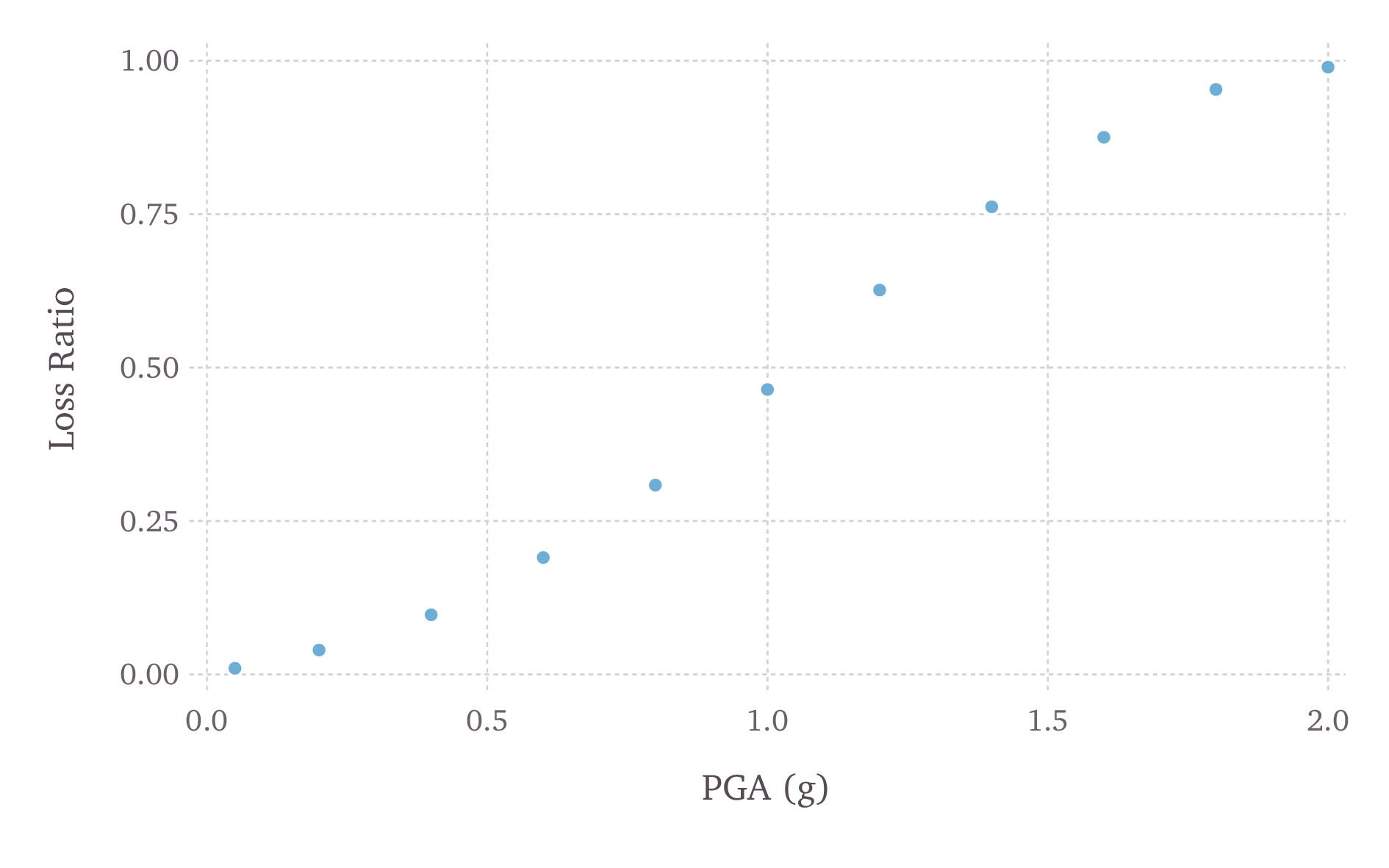
Fig. 3.10 Graphical representation of a vulnerability model#
Note that although the uncertainty for each loss ratio is not represented in Fig. 3.10, it can be considered in the input file, by means of a coefficient of variation per loss ratio and a probabilistic distribution, which can currently be set to lognormal (LN), Beta (BT); or by specifying a discrete probability mass (PM) 4 distribution of the loss ratio at a set of intensity levels. An example of a Vulnerability Function that models the uncertainty in the loss ratio at different intensity levels using a lognormal distribution is illustrated in Fig. 3.11.
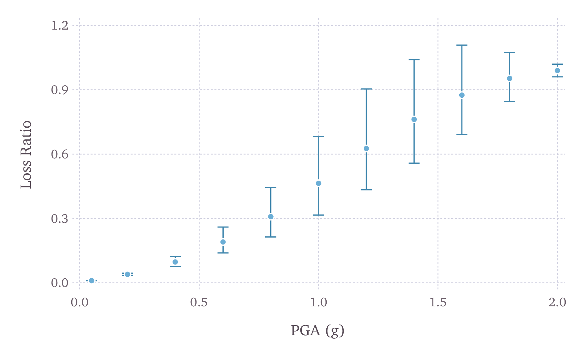
Fig. 3.11 Graphical representation of a vulnerability function that models the uncertainty in the loss ratio using a lognormal distribution. The mean loss ratios and coefficients of variation are illustrated for a set of intensity levels.#
In general, defining vulnerabilityfunctions requires the user to specify the distribution of the loss ratio for a set of intensity levels. The loss ratio distributions can be defined using either a discrete or a continuous format, and the Vulnerability Model file can include a mix of both types of vulnerabilityfunctions. It is also possible to define a Vulnerability Function using a set of deterministic loss ratios corresponding to a set of intensity levels (i.e., ignoring the uncertainty in the conditional loss ratios).
An example Vulnerability Model comprising three vulnerability functions is shown in the listing below. This Vulnerability Model contains one function that uses the lognormal distribution to represent the uncertainty in the loss ratio at different intensity levels, one function that uses the Beta distribution, and one function that is defined using a discrete probability mass distribution.
 1<?xml version="1.0" encoding="UTF-8"?>
 2<nrml xmlns="http://openquake.org/xmlns/nrml/0.5">
 3
 4<vulnerabilityModel id="vulnerability_example"
 5                    assetCategory="buildings"
 6                    lossCategory="structural">
 7
 8  <description>vulnerability model</description>
 9
10  <vulnerabilityFunction id="W1_Res_LowCode" dist="LN">
11   <imls imt="PGA">0.005 0.15 0.4 0.6 0.8 1.0 1.2 1.4 1.6 1.8 2.0</imls>
12   <meanLRs>0.01 0.04 0.10 0.20 0.33 0.50 0.67 0.80 0.90 0.96 0.99</meanLRs>
13   <covLRs>0.03 0.12 0.24 0.32 0.38 0.40 0.38 0.32 0.24 0.12 0.03</covLRs>
14  </vulnerabilityFunction>
15
16
17  <vulnerabilityFunction id="S1_Res_HighCode" dist="BT">
18   <imls imt="SA(0.3)">0.05 0.2 0.4 0.6 0.8 1.0 1.2 1.4 1.6 1.8 2.0</imls>
19   <meanLRs>0.01 0.03 0.07 0.15 0.24 0.37 0.50 0.60 0.67 0.72 0.75</meanLRs>
20   <covLRs>0.03 0.12 0.24 0.32 0.38 0.40 0.38 0.32 0.24 0.12 0.03</covLRs>
21  </vulnerabilityFunction>
22
23
24  <vulnerabilityFunction id="ATC13_URM_Res" dist="PM">
25   <imls imt="MMI">6 7 8 9 10 11 12</imls>
26   <probabilities lr="0.000">0.95 0.49 0.30 0.14 0.03 0.01 0.00</probabilities>
27   <probabilities lr="0.005">0.03 0.38 0.40 0.30 0.10 0.03 0.01</probabilities>
28   <probabilities lr="0.050">0.02 0.08 0.16 0.24 0.30 0.10 0.01</probabilities>
29   <probabilities lr="0.200">0.00 0.02 0.08 0.16 0.26 0.30 0.03</probabilities>
30   <probabilities lr="0.450">0.00 0.02 0.03 0.10 0.18 0.30 0.18</probabilities>
31   <probabilities lr="0.800">0.00 0.01 0.02 0.04 0.10 0.18 0.39</probabilities>
32   <probabilities lr="1.000">0.00 0.01 0.01 0.02 0.03 0.08 0.38</probabilities>
33  </vulnerabilityFunction>
34
35</vulnerabilityModel>
36
37</nrml>
The initial portion of the schema contains general information that describes some general aspects of the Vulnerability Model. The information in this metadata section is common to all of the functions in the Vulnerability Model and needs to be included at the beginning of every Vulnerability Model file. The parameters are illustrated in the snippet shown and described below:
4<vulnerabilityModel id="vulnerability_example"
5                    assetCategory="buildings"
6                    lossCategory="structural">
7
8  <description>vulnerability model</description>
id: a unique string (ASCII) used to identify the Vulnerability Model. This string can contain letters (a–z; A–Z), numbers (0–9), dashes (-), and underscores (_), with a maximum of 100 characters.assetCategory: an optional string (ASCII) used to specify the type of assets for which vulnerabilityfunctions will be defined in this file (e.g: buildings, lifelines).lossCategory: mandatory; valid strings for this attribute are “structural”, “nonstructural”, “contents”, “business_interruption”, and “occupants”.description: mandatory; a brief string with further information about the Vulnerability Model, for example, which building typologies are covered or the source of the functions in the Vulnerability Model.
The following snippet from the above Vulnerability Model example file defines a Vulnerability Function modelling the uncertainty in the conditional loss ratios using a (continuous) lognormal distribution:
10  <vulnerabilityFunction id="W1_Res_LowCode" dist="LN">
11   <imls imt="PGA">0.005 0.15 0.4 0.6 0.8 1.0 1.2 1.4 1.6 1.8 2.0</imls>
12   <meanLRs>0.01 0.04 0.10 0.20 0.33 0.50 0.67 0.80 0.90 0.96 0.99</meanLRs>
13   <covLRs>0.03 0.12 0.24 0.32 0.38 0.40 0.38 0.32 0.24 0.12 0.03</covLRs>
14  </vulnerabilityFunction>
The following attributes are needed to define a Vulnerability Function which uses a continuous distribution to model the uncertainty in the conditional loss ratios:
id: a unique string (ASCII) used to identify the taxonomy for which the function is being defined. This string is used to relate the Vulnerability Function with the relevant asset in the Exposure Model. This string can contain letters (a–z; A–Z), numbers (0–9), dashes (-), and underscores (_), with a maximum of 100 characters.dist: mandatory; for vulnerabilityfunctions which use a continuous distribution to model the uncertainty in the conditional loss ratios, this attribute should be set to either “LN” if using the lognormal distribution, or to “BT” if using the Beta distribution.imls: mandatory; this attribute specifies the list of intensity levels for which the parameters of the conditional loss ratio distributions will be defined. In addition, it is also necessary to define the intensity measure type (imt).meanLRs: mandatory; this field is used to define the mean loss ratios for this Vulnerability Function for each of the intensity levels defined by the attributeimls. The number of mean loss ratios defined by themeanLRsattribute must be equal to the number of intensity levels defined by the attributeimls.covLRs: mandatory; this field is used to define the coefficient of variation for the conditional distribution of the loss ratios for this Vulnerability Function for each of the intensity levels defined by the attributeimls. The number of coefficients of variation of loss ratios defined by thecovLRsattribute must be equal to the number of intensity levels defined by the attributeimls. The uncertainty in the conditional loss ratios can be ignored by setting all of thecovLRsfor a given Vulnerability Function to zero.
The next snippet from the Vulnerability Model example file of the Vulnerability Function listing above defines a Vulnerability Function which models the uncertainty in the conditional loss ratios using a (discrete) probability mass distribution:
24  <vulnerabilityFunction id="ATC13_URM_Res" dist="PM">
25   <imls imt="MMI">6 7 8 9 10 11 12</imls>
26   <probabilities lr="0.000">0.95 0.49 0.30 0.14 0.03 0.01 0.00</probabilities>
27   <probabilities lr="0.005">0.03 0.38 0.40 0.30 0.10 0.03 0.01</probabilities>
28   <probabilities lr="0.050">0.02 0.08 0.16 0.24 0.30 0.10 0.01</probabilities>
29   <probabilities lr="0.200">0.00 0.02 0.08 0.16 0.26 0.30 0.03</probabilities>
30   <probabilities lr="0.450">0.00 0.02 0.03 0.10 0.18 0.30 0.18</probabilities>
31   <probabilities lr="0.800">0.00 0.01 0.02 0.04 0.10 0.18 0.39</probabilities>
32   <probabilities lr="1.000">0.00 0.01 0.01 0.02 0.03 0.08 0.38</probabilities>
33  </vulnerabilityFunction>
The following attributes are needed to define a Vulnerability Function which uses a discrete probability mass distribution to model the uncertainty in the conditional loss ratios:
id: a unique string (ASCII) used to identify the taxonomy for which the function is being defined. This string is used to relate the Vulnerability Function with the relevant asset in the Exposure Model. This string can contain letters (a–z; A–Z), numbers (0–9), dashes (-), and underscores (_), with a maximum of 100 characters.dist: mandatory; for vulnerabilityfunctions which use a discrete probability mass distribution to model the uncertainty in the conditional loss ratios, this attribute should be set to “PM”.imls: mandatory; this attribute specifies the list of intensity levels for which the parameters of the conditional loss ratio distributions will be defined. In addition, it is also necessary to define the intensity measure type (imt).probabilities: mandatory; this field is used to define the probability of observing a particular loss ratio (specified for each row ofprobabilitiesusing the attributelr), conditional on the set of intensity levels specified using the attributeimls. for this Vulnerability Function. Thus, the number of probabilities defined by eachprobabilitiesattribute must be equal to the number of intensity levels defined by the attributeimls. On the other hand, there is no limit to the number of loss ratios for whichprobabilitiescan be defined. In the example shown here, notice that the set of probabilities conditional on any particular intensity level, say, \(MMI = 8\), sum up to one.
Note that the schema for representing vulnerabilitymodels has changed between Natural hazards’ Risk Markup Language v0.4 (used prior to OpenQuake engine17) and Natural hazards’ Risk Markup Language v0.5 (introduced in OpenQuake engine17).
A deprecation warning is printed every time you attempt to use a
Vulnerability Model in the old Natural hazards’ Risk Markup Language v0.4 format in an OpenQuake engine17 (or
later) risk calculation. To get rid of the warning you must upgrade the
old vulnerabilitymodels files to Natural hazards’ Risk Markup Language v0.5. You can use the command
upgrade_nrml with oq to do this as follows:
user@ubuntu:~$ oq upgrade_nrml <directory-name>
The above command will upgrade all of your old Vulnerability Model files
to Natural hazards’ Risk Markup Language v0.5. The original files will be kept, but with a .bak
extension appended. Notice that you will need to set the
lossCategory attribute to its correct value manually. This is easy
to do, since if you try to run a computation you will get a clear error
message telling the expected value for the lossCategory for each
file.
Several methodologies to derive vulnerabilityfunctions are currently being evaluated by GEM Foundation and have been included as part of the Risk Modeller’s Toolkit, the code for which can be found on a public repository at GitHub at: gemsciencetools/rmtk.
A web-based tool to build an Vulnerability Model in the Natural hazards’ Risk Markup Language schema are also under development, and can be found at the OpenQuake platform at the following address: https://platform.openquake.org/ipt/.
3.3. Using the Risk Module#
This Chapter summarises the structure of the information necessary to define the different input data to be used with the OpenQuake engine risk calculators. Input data for scenario-based and probabilistic seismic damage and risk analysis using the OpenQuake engine are organised into:
An exposure model file in the NRML format, as described in Section Exposure Models.
A file describing the Vulnerability Model (Section Vulnerability Models) for loss calculations, or a file describing the Fragility Model (Section Fragility Models) for damage calculations. Optionally, a file describing the Consequence Model (Section Consequence Models) can also be provided in order to calculate losses from the estimated damage distributions.
A general calculation configuration file.
Hazard inputs. These include hazard curves for the classical probabilistic damage and risk calculators, ground motion fields for the scenario damage and risk calculators, or stochastic event sets for the probabilistic event based calculators. As of OpenQuake engine21, in general, there are five different ways in which hazard calculation parameters or results can be provided to the OpenQuake engine in order to run the subsequent risk calculations:
Use a single configuration file for running the hazard and risk calculations sequentially (preferred)
Use separate configuration files for running the hazard and risk calculations sequentially (legacy)
Use a configuration file for the risk calculation along with all hazard outputs from a previously completed, compatible OpenQuake engine hazard calculation
Use a configuration file for the risk calculation along with hazard input files in the OpenQuake NRML format
The file formats for Exposure models, Fragility Models, Consequence Models, and Vulnerability models have been described earlier in Chapter Risk Input Models. The configuration file is the primary file that provides the OpenQuake engine information regarding both the definition of the input models (e.g. exposure, site parameters, fragility, consequence, or vulnerability models) as well as the parameters governing the risk calculation.
Information regarding the configuration file for running hazard calculations using the OpenQuake engine can be found in Section Configuration file. Some initial mandatory parameters of the configuration file common to all of the risk calculators are presented in the listing. The remaining parameters that are specific to each risk calculator are discussed in subsequent sections.
[general]
description = Example risk calculation
calculation_mode = scenario_risk

[exposure]
exposure_file = exposure_model.xml

[vulnerability]
structural_vulnerability_file = structural_vulnerability_model.xml
description: a parameter that can be used to include some information about the type of calculations that are going to be performed.calculation_mode: this parameter specifies the type of calculation to be run. Valid options for thecalculation_modefor the risk calculators are:scenario_damage,scenario_risk,classical_damage,classical_risk,event_based_risk, andclassical_bcr.exposure_file: this parameter is used to specify the path to the Exposure Model file. Typically this is the path to the xml file containing the exposure, or the xml file containing the metadata sections for the case where the assets are listed in one or more csv files. For particularly large exposure models, it may be more convenient to provide the path to a single compressed zip file that contains the exposure xml file and the exposure csv files (if any).
Depending on the type of risk calculation, other parameters besides the aforementioned ones may need to be provided. We illustrate in the following sections different examples of the configuration file for the different risk calculators.
3.3.1. Scenario Damage Calculator#
For this calculator,
the parameter calculation_mode should be set to scenario_damage.
Example 1
This example illustrates a scenario damage calculation which uses a single configuration file to first compute the ground motion fields for the given rupture model and then calculate damage distribution statistics based on the ground motion fields. A minimal job configuration file required for running a scenario damage calculation is shown in the listing below.
[general]
description = Scenario damage using a single config file
calculation_mode = scenario_damage

[exposure]
exposure_file = exposure_model.xml

[rupture]
rupture_model_file = rupture_model.xml
rupture_mesh_spacing = 2.0

[site_params]
site_model_file = site_model.xml

[hazard_calculation]
random_seed = 42
truncation_level = 3.0
maximum_distance = 200.0
gsim = BooreAtkinson2008
number_of_ground_motion_fields = 1000

[fragility]
structural_fragility_file = structural_fragility_model.xml
The general parameters description and calculation_mode, and
exposure_file have already been described earlier. The other
parameters seen in the above example configuration file are described
below:
rupture_model_file: a parameter used to define the path to the earthquake Rupture Model file describing the scenario event.rupture_mesh_spacing: a parameter used to specify the mesh size (in km) used by the OpenQuake engine to discretize the rupture. Note that the smaller the mesh spacing, the greater will be (1) the precision in the calculation and (2) the computational demand.structural_fragility_file: a parameter used to define the path to the structural Fragility Model file.
In this case, the ground motion fields will be computed at each of the locations of the assets in the exposure model. Ground motion fields will be generated for each of the intensity measure types found in the provided set of fragility models. The above calculation can be run using the command line:
user@ubuntu:~$ oq engine --run job.ini
After the calculation is completed, a message similar to the following will be displayed:
Calculation 2680 completed in 13 seconds. Results:
  id | name
5069 | Average Asset Damages
Note that one or more of the following parameters can be used in the same job configuration file to provide the corresponding fragility model files:
structural_fragility_file: a parameter used to define the path to a structural Fragility Model filenonstructural_fragility_file: a parameter used to define the path to a nonstructural Fragility Model filecontents_fragility_file: a parameter used to define the path to a contents Fragility Model filebusiness_interruption_fragility_file: a parameter used to define the path to a business interruption Fragility Model file
It is important that the lossCategory parameter in the metadata
section for each provided fragility model file (“structural”,
“nonstructural”, “contents”, or “business_interruption”) should match
the loss type defined in the configuration file by the relevant keyword
above.
Example 2
This example illustrates a scenario damage calculation which uses separate configuration files for the hazard and risk parts of a scenario damage assessment. The first configuration file shown in the first listing below contains input models and parameters required for the computation of the ground motion fields due to a given rupture. The second configuration file shown in the second listing contains input models and parameters required for the calculation of the damage distribution for a portfolio of assets due to the ground motion fields.
Scenario hazard example
[general]
description = Scenario hazard example
calculation_mode = scenario

[rupture]
rupture_model_file = rupture_model.xml
rupture_mesh_spacing = 2.0

[sites]
sites_csv = sites.csv

[site_params]
site_model_file = site_model.xml

[hazard_calculation]
random_seed = 42
truncation_level = 3.0
maximum_distance = 200.0
gsim = BooreAtkinson2008
intensity_measure_types = PGA, SA(0.3)
number_of_ground_motion_fields = 1000
ground_motion_correlation_model = JB2009
ground_motion_correlation_params = {"vs30_clustering": True}
Scenario damage example
[general]
description = Scenario damage example
calculation_mode = scenario_damage

[exposure]
exposure_file = exposure_model.xml

[boundaries]
region = -123.0 38.3, -121.0 38.3, -121.0 36.5, -123.0 36.5

[hazard]
asset_hazard_distance = 20

[fragility]
structural_fragility_file = structural_fragility_model.xml

[risk_calculation]
time_event = night
In this example, the set of intensity measure types for which the ground
motion fields should be generated is specified explicitly in the
configuration file using the parameter intensity_measure_types. If
the hazard calculation outputs are intended to be used as inputs for a
subsequent scenario damage or risk calculation, the set of intensity
measure types specified here must include all intensity measure types
that are used in the fragility or vulnerability models for the
subsequent damage or risk calculation.
In
the hazard configuration file
illustrated above,
the list of sites at which the ground motion values will be computed is
provided in a CSV file, specified using the sites_csv parameter. The
sites used for the hazard calculation need not be the same as the
locations of the assets in the exposure model used for the following
risk calculation. In such cases, it is recommended to set a reasonable
search radius (in km) using the asset_hazard_distance parameter for
the OpenQuake engine to look for available hazard values, as shown in the
job_damage.ini example file above.
The only new parameters introduced in
the risk configuration file
for this example
are the region, asset_hazard_distance, and time_event
parameters, which are described below; all other parameters have already
been described in earlier examples.
region: this is an optional parameter which defines the polygon that will be used for filtering the assets from the exposure model. Assets outside of this region will not be considered in the risk calculations. This region is defined using pairs of coordinates that indicate the vertices of the polygon, which should be listed in the Well-known text (WKT) format:region = lon_1 lat_1, lon_2 lat_2, …, lon_n lat_n
For each point, the longitude is listed first, followed by the latitude, both in decimal degrees. The list of points defining the polygon can be provided either in a clockwise or counter-clockwise direction.
If the
regionis not provided, all assets in the exposure model are considered for the risk calculation.This parameter is useful in cases where the exposure model covers a region larger than the one that is of interest in the current calculation.
asset_hazard_distance: this parameter indicates the maximum allowable distance between an asset and the closest hazard input. Hazard inputs can include hazard curves or ground motion intensity values. If no hazard input site is found within the radius defined by theasset_hazard_distance, the asset is skipped and a message is provided mentioning the id of the asset that is affected by this issue.If multiple hazard input sites are found within the radius defined by the this parameter, the hazard input site with the shortest distance from the asset location is associated with the asset. It is possible that the associated hazard input site might be located outside the polygon defined by the
region.time_event: this parameter indicates the time of day at which the event occurs. The values that this parameter can be set to are currently limited to one of the three strings:day,night, andtransit. This parameter will be used to compute the number of fatalities based on the number of occupants present in the various assets at that time of day, as specified in the exposure model.
Now, the above calculations described by the two configuration files
“job_hazard.ini” and “job_damage.ini” can be run separately. The
calculation id for the hazard calculation should be provided to the
OpenQuake engine while running the risk calculation using the option
--hazard-calculation-id (or --hc). This is shown below:
user@ubuntu:~$ oq engine --run job_hazard.ini
After the hazard calculation is completed, a message similar to the one below will be displayed in the terminal:
Calculation 2681 completed in 4 seconds. Results:
  id | name
5072 | Ground Motion Fields
In the example above, the calculation id of the hazard calculation is 2681. There is only one output from this calculation, i.e., the Ground Motion Fields.
The risk calculation for computing the damage distribution statistics for the portfolio of assets can now be run using:
user@ubuntu:~$ oq engine --run job_damage.ini --hc 2681
After the calculation is completed, a message similar to the one listed above in Example 1 will be displayed.
In order to retrieve the calculation id of a previously run hazard
calculation, the option --list-hazard-calculations (or --lhc)
can be used to display a list of all previously run hazard calculations:
job_id |     status |         start_time |         description
  2609 | successful | 2015-12-01 14:14:14 | Mid Nepal earthquake
  ...
  2681 | successful | 2015-12-12 10:00:00 | Scenario hazard example
The option --list-outputs (or --lo) can be used to display a
list of all outputs generated during a particular calculation. For
instance,
user@ubuntu:~$ oq engine --lo 2681
will produce the following display:
  id | name
5072 | Ground Motion Fields
Example 3
The example shown in the listing below illustrates a scenario damage calculation which uses a file listing a precomputed set of Ground Motion Fields. These Ground Motion Fields can be computed using the OpenQuake engine or some other software. The Ground Motion Fields must be provided in either the Natural hazards’ Risk Markup Language schema or the csv format as presented in Section Outputs from Scenario Hazard Analysis. The damage distribution is computed based on the provided Ground Motion Fields.
[general]
description = Scenario damage using user-defined ground motion fields (NRML)
calculation_mode = scenario_damage

[hazard]
gmfs_file = gmfs.xml

[exposure]
exposure_file = exposure_model.xml

[fragility]
structural_fragility_file = structural_fragility_model.xml
gmfs_file: a parameter used to define the path to the Ground Motion Fields file in the Natural hazards’ Risk Markup Language schema. This file must define Ground Motion Fields for all of the intensity measure types used in the Fragility Model.
The listing below
shows an example of a Ground Motion Fields file in the Natural hazards’
Risk Markup Language schema and
Table 2.3 shows an example of a Ground Motion Fields file
in the csv format. If the Ground Motion Fields file is provided in the csv format,
an additional csv file listing the site ids must be provided using the
parameter sites_csv. See Table 2.4 for an
example of the sites csv file, which provides the association between
the site ids in the Ground Motion Fields csv file with their latitude and longitude
coordinates.
[general]
description = Scenario damage using user-defined ground motion fields (CSV)
calculation_mode = scenario_damage

[hazard]
sites_csv = sites.csv
gmfs_csv = gmfs.csv

[exposure]
exposure_file = exposure_model.xml

[fragility]
structural_fragility_file = structural_fragility_model.xml
gmfs_csv: a parameter used to define the path to the Ground Motion Fields file in the csv format. This file must define Ground Motion Fields for all of the intensity measure types used in the Fragility Model. (Download an example file here).sites_csv: a parameter used to define the path to the sites file in the csv format. This file must define site id, longitude, and latitude for all of the sites for the Ground Motion Fields file provided using thegmfs_csvparameter. (Download an example file here).
The above calculation(s) can be run using the command line:
user@ubuntu:~$ oq engine --run job.ini
Example 4
This example illustrates a the hazard job configuration file for a scenario damage calculation which uses two Ground Motion Prediction Equations instead of only one. Currently, the set of Ground Motion Prediction Equations to be used for a scenario calculation can be specified using a logic tree file, as demonstrated in The Ground Motion Logic Tree. As of OpenQuake engine18, the weights in the logic tree are ignored, and a set of Ground Motion Fields will be generated for each Ground Motion Prediction Equation in the logic tree file. Correspondingly, damage distribution statistics will be generated for each set of Ground Motion Field.
The file shown in the listing below lists the two Ground Motion Prediction Equations to be used for the hazard calculation:
 1<?xml version="1.0" encoding="UTF-8"?>
 2<nrml xmlns:gml="http://www.opengis.net/gml"
 3      xmlns="http://openquake.org/xmlns/nrml/0.5">
 4
 5<logicTree logicTreeID="lt1">
 6    <logicTreeBranchSet uncertaintyType="gmpeModel"
 7                        branchSetID="bs1"
 8                        applyToTectonicRegionType="Active Shallow Crust">
 9
10      <logicTreeBranch branchID="b1">
11        <uncertaintyModel>BooreAtkinson2008</uncertaintyModel>
12        <uncertaintyWeight>0.75</uncertaintyWeight>
13      </logicTreeBranch>
14
15      <logicTreeBranch branchID="b2">
16        <uncertaintyModel>ChiouYoungs2008</uncertaintyModel>
17        <uncertaintyWeight>0.25</uncertaintyWeight>
18      </logicTreeBranch>
19
20    </logicTreeBranchSet>
21</logicTree>
22
23</nrml>
The only change that needs to be made in the hazard job configuration
file is to replace the gsim parameter with gsim_logic_tree_file,
as demonstrated in
the listing below.
[general]
description = Scenario hazard example using multiple GMPEs
calculation_mode = scenario

[rupture]
rupture_model_file = rupture_model.xml
rupture_mesh_spacing = 2.0

[sites]
sites_csv = sites.csv

[site_params]
site_model_file = site_model.xml

[hazard_calculation]
random_seed = 42
truncation_level = 3.0
maximum_distance = 200.0
gsim_logic_tree_file = gsim_logic_tree.xml
intensity_measure_types = PGA, SA(0.3)
number_of_ground_motion_fields = 1000
ground_motion_correlation_model = JB2009
ground_motion_correlation_params = {"vs30_clustering": True}
Example 5
This example illustrates a scenario damage calculation which specifies fragility models for calculating damage to structural and nonstructural components of structures, and also specifies Consequence Model files for calculation of the corresponding losses.
A minimal job configuration file required for running a scenario damage calculation followed by a consequences analysis is shown in the listing below.
[general]
description = Scenario damage and consequences
calculation_mode = scenario_damage

[exposure]
exposure_file = exposure_model.xml

[rupture]
rupture_model_file = rupture_model.xml
rupture_mesh_spacing = 2.0

[site_params]
site_model_file = site_model.xml

[hazard_calculation]
random_seed = 42
truncation_level = 3.0
maximum_distance = 200.0
gsim = BooreAtkinson2008
number_of_ground_motion_fields = 1000
ground_motion_correlation_model = JB2009
ground_motion_correlation_params = {"vs30_clustering": True}

[fragility]
structural_fragility_file = structural_fragility_model.xml
nonstructural_fragility_file = nonstructural_fragility_model.xml

[consequence]
structural_consequence_file = structural_consequence_model.xml
nonstructural_consequence_file = nonstructural_consequence_model.xml
Note that one or more of the following parameters can be used in the same job configuration file to provide the corresponding Consequence Model files:
structural_consequence_file: a parameter used to define the path to a structural Consequence Model filenonstructural_consequence_file: a parameter used to define the path to a nonstructural Consequence Model filecontents_consequence_file: a parameter used to define the path to a contents Consequence Model filebusiness_interruption_consequence_file: a parameter used to define the path to a business interruption Consequence Model file
It is important that the lossCategory parameter in the metadata
section for each provided Consequence Model file (“structural”,
“nonstructural”, “contents”, or “business_interruption”) should match
the loss type defined in the configuration file by the relevant keyword
above.
The above calculation can be run using the command line:
user@ubuntu:~$ oq engine --run job.ini
After the calculation is completed, a message similar to the following will be displayed:
Calculation 1579 completed in 37 seconds. Results:
  id | name
8990 | Average Asset Losses
8993 | Average Asset Damages
3.3.2. Scenario Risk Calculator#
In order to run this
calculator, the parameter calculation_mode needs to be set to
scenario_risk.
Most of the job configuration parameters required for running a scenario risk calculation are the same as those described in the previous section for the scenario damage calculator. The remaining parameters specific to the scenario risk calculator are illustrated through the examples below.
Example 1
This example illustrates a scenario risk calculation which uses a single configuration file to first compute the ground motion fields for the given rupture model and then calculate loss statistics for structural losses and nonstructural losses, based on the ground motion fields. The job configuration file required for running this scenario risk calculation is shown in the listing below.
[general]
description = Scenario risk using a single config file
calculation_mode = scenario_risk

[exposure]
exposure_file = exposure_model.xml

[rupture]
rupture_model_file = rupture_model.xml
rupture_mesh_spacing = 2.0

[site_params]
site_model_file = site_model.xml

[hazard_calculation]
random_seed = 42
truncation_level = 3.0
maximum_distance = 200.0
gsim = BooreAtkinson2008
number_of_ground_motion_fields = 1000
ground_motion_correlation_model = JB2009
ground_motion_correlation_params = {"vs30_clustering": True}

[vulnerability]
structural_vulnerability_file = structural_vulnerability_model.xml
nonstructural_vulnerability_file = nonstructural_vulnerability_model.xml

[risk_calculation]
master_seed = 24
asset_correlation = 1
Whereas a scenario damage calculation requires one or more fragility and/or consequence models, a scenario risk calculation requires the user to specify one or more vulnerability model files. Note that one or more of the following parameters can be used in the same job configuration file to provide the corresponding vulnerability model files:
structural_vulnerability_file: this parameter is used to specify the path to the structural Vulnerability Model filenonstructural_vulnerability_file: this parameter is used to specify the path to the nonstructuralvulnerabilitymodel filecontents_vulnerability_file: this parameter is used to specify the path to the contents Vulnerability Model filebusiness_interruption_vulnerability_file: this parameter is used to specify the path to the business interruption Vulnerability Model fileoccupants_vulnerability_file: this parameter is used to specify the path to the occupants Vulnerability Model file
It is important that the lossCategory parameter in the metadata
section for each provided vulnerability model file (“structural”,
“nonstructural”, “contents”, “business_interruption”, or “occupants”)
should match the loss type defined in the configuration file by the
relevant keyword above.
The remaining new parameters introduced in this example are the following:
master_seed: this parameter is used to control the random number generator in the loss ratio sampling process. If the samemaster_seedis defined at each calculation run, the same random loss ratios will be generated, thus allowing reproducibility of the results.asset_correlation: if the uncertainty in the loss ratios has been defined within the Vulnerability Model, users can specify a coefficient of correlation that will be used in the Monte Carlo sampling process of the loss ratios, between the assets that share the same taxonomy. If theasset_correlationis set to one, the loss ratio residuals will be perfectly correlated. On the other hand, if this parameter is set to zero, the loss ratios will be sampled independently. If this parameter is not defined, the OpenQuake engine will assume zero correlation in the vulnerability. As of OpenQuake engine18,asset_correlationapplies only to continuous vulnerabilityfunctions using the lognormal or Beta distribution; it does not apply to vulnerabilityfunctions defined using the PMF distribution. Although partial correlation was supported in previous versions of the engine, beginning from OpenQuake engine22, values between zero and one are no longer supported due to performance considerations. The only two values permitted areasset_correlation = 0andasset_correlation = 1.
In this case, the ground motion fields will be computed at each of the locations of the assets in the exposure model and for each of the intensity measure types found in the provided set of vulnerability models. The above calculation can be run using the command line:
user@ubuntu:~$ oq engine --run job.ini
After the calculation is completed, a message similar to the following will be displayed:
Calculation 2735 completed in 10 seconds. Results:
  id | name
5328 | Aggregate Asset Losses
5329 | Average Asset Losses
5330 | Aggregate Event Losses
All of the different ways of running a scenario damage calculation as illustrated through the examples of the previous section are also applicable to the scenario risk calculator, though the examples are not repeated here.
A few additional parameters related to the event based risk calculator that may be useful for controlling specific aspects of the calculation are listed below:
ignore_covs: this parameter controls the propagation of vulnerability uncertainty to losses. The vulnerability functions using continuous distributions (such as the lognormal distribution or beta distribution) to characterize the uncertainty in the loss ratio conditional on the shaking intensity level, specify the mean loss ratios and the corresponding coefficients of variation for a set of intensity levels. They are used to build the so called Epsilon matrix within the engine, which is how loss ratios are sampled from the distribution for each asset. There is clearly a performance penalty associated with the propagation of uncertainty in the vulnerability to losses. The Epsilon matrix has to be computed and stored, and then the worker processes have to read it, which involves large quantities of data transfer and memory usage. Settingignore_covs = truein the job file will result in the engine using just the mean loss ratio conditioned on the shaking intensity and ignoring the uncertainty. This tradeoff of not propagating the vulnerabilty uncertainty to the loss estimates can lead to a significant boost in performance and tractability. The default value ofignore_covsisfalse.
3.3.3. Classical Probabilistic Seismic Damage Calculator#
In order to run this calculator, the parameter
calculation_mode needs to be set to classical_damage.
Most of the job configuration parameters required for running a classical probabilistic damage calculation are the same as those described in the section for the scenario damage calculator. The remaining parameters specific to the classical probabilistic damage calculator are illustrated through the examples below.
Example 1
This example illustrates a classical probabilistic damage calculation which uses a single configuration file to first compute the hazard curves for the given source model and ground motion model and then calculate damage distribution statistics based on the hazard curves. A minimal job configuration file required for running a classical probabilistic damage calculation is shown in the listing below.
[general]
description = Classical probabilistic damage using a single config file
calculation_mode = classical_damage

[exposure]
exposure_file = exposure_model.xml

[erf]
width_of_mfd_bin = 0.1
rupture_mesh_spacing = 2
area_source_discretization = 20

[site_params]
site_model_file = site_model.xml

[logic_trees]
source_model_logic_tree_file = source_model_logic_tree.xml
gsim_logic_tree_file = gsim_logic_tree.xml
number_of_logic_tree_samples = 0

[hazard_calculation]
random_seed = 42
investigation_time = 1
truncation_level = 3.0
maximum_distance = 200.0

[fragility]
structural_fragility_file = structural_fragility_model.xml
The general parameters description and calculation_mode, and
exposure_file have already been described earlier in
Section Scenario Damage Calculator.
The parameters related to the hazard curves computation have been
described earlier in
Section Classical PSHA.
In this case, the hazard curves will be computed at each of the locations of the assets in the exposure model, for each of the intensity measure types found in the provided set of fragilitymodels. The above calculation can be run using the command line:
user@ubuntu:~$ oq engine --run job.ini
After the calculation is completed, a message similar to the following will be displayed:
Calculation 2741 completed in 12 seconds. Results:
  id | name
5359 | Asset Damage Distribution
Example 2
This example illustrates a classical probabilistic damage calculation which uses separate configuration files for the hazard and risk parts of a classical probabilistic damage assessment. The first configuration file shown in the listing below contains input models and parameters required for the computation of the hazard curves.
[general]
description = Classical probabilistic hazard
calculation_mode = classical

[sites]
region = -123.0 38.3, -121.0 38.3, -121.0 36.5, -123.0 36.5
region_grid_spacing = 0.5

[erf]
width_of_mfd_bin = 0.1
rupture_mesh_spacing = 2
area_source_discretization = 20

[site_params]
site_model_file = site_model.xml

[logic_trees]
source_model_logic_tree_file = source_model_logic_tree.xml
gsim_logic_tree_file = gsim_logic_tree.xml
number_of_logic_tree_samples = 0

[hazard_calculation]
random_seed = 42
investigation_time = 1
truncation_level = 3.0
maximum_distance = 200.0
intensity_measure_types_and_levels = {
 "PGA": logscale(0.05, 3.0, 30),
 "SA(1.0)": logscale(0.05, 3.0, 30)}
The second configuration file shown in the listing below contains input models and parameters required for the calculation of the probabilistic damage distribution for a portfolio of assets based on the hazard curves and fragility models.
[general]
description = Classical probabilistic damage example
calculation_mode = classical_damage

[exposure]
exposure_file = exposure_model.xml

[hazard]
asset_hazard_distance = 20

[fragility]
structural_fragility_file = structural_fragility_model.xml

[risk_calculation]
risk_investigation_time = 50
steps_per_interval = 4
Now, the above calculations described by the two configuration files “job_hazard.ini” and “job_damage.ini” can be run sequentially or separately, as illustrated in Example 2 in Section Scenario Damage Calculator. The new parameters introduced in the above example configuration file are described below:
risk_investigation_time: an optional parameter that can be used in probabilistic damage or risk calculations where the period of interest for the risk calculation is different from the period of interest for the hazard calculation. If this parameter is not explicitly set, the OpenQuake engine will assume that the risk calculation is over the same time period as the preceding hazard calculation.steps_per_interval: an optional parameter that can be used to specify whether discrete fragility functions in the fragility models should be discretized further, and if so, how many intermediate steps to use for the discretization. Settingsteps_per_interval = n
will result in the OpenQuake engine discretizing the discrete fragility models using (n - 1) linear interpolation steps between each pair of intensity level, poe points.
The default value of this parameter is one, implying no interpolation.
3.3.4. Classical Probabilistic Seismic Risk Calculator#
In order to run this calculator, the parameter calculation_mode
needs to be set to classical_risk.
Most of the job configuration parameters required for running a classical probabilistic risk calculation are the same as those described in the previous section for the classical probabilistic damage calculator. The remaining parameters specific to the classical probabilistic risk calculator are illustrated through the examples below.
Example 1
This example illustrates a classical probabilistic risk calculation which uses a single configuration file to first compute the hazard curves for the given source model and ground motion model and then calculate loss exceedance curves based on the hazard curves. An example job configuration file for running a classical probabilistic risk calculation is shown in the listing below.
[general]
description = Classical probabilistic risk using a single config file
calculation_mode = classical_risk

[exposure]
exposure_file = exposure_model.xml

[erf]
width_of_mfd_bin = 0.1
rupture_mesh_spacing = 2
area_source_discretization = 20

[site_params]
site_model_file = site_model.xml

[logic_trees]
source_model_logic_tree_file = source_model_logic_tree.xml
gsim_logic_tree_file = gsim_logic_tree.xml
number_of_logic_tree_samples = 0

[hazard_calculation]
random_seed = 42
investigation_time = 1
truncation_level = 3.0
maximum_distance = 200.0

[vulnerability]
structural_vulnerability_file = structural_vulnerability_model.xml
nonstructural_vulnerability_file = nonstructural_vulnerability_model.xml
Apart from the calculation mode, the only difference with the example job configuration file shown in Example 1 of Section Classical Probabilistic Seismic Damage Calculator is the use of a vulnerability model instead of a fragility model.
As with the Scenario Risk calculator, it is possible to specify one or more Vulnerability Model files in the same job configuration file, using the parameters:
structural_vulnerability_file,nonstructural_vulnerability_file,contents_vulnerability_file,business_interruption_vulnerability_file, and/oroccupants_vulnerability_file
It is important that the lossCategory parameter in the metadata
section for each provided vulnerability model file (“structural”,
“nonstructural”, “contents”, “business_interruption”, or “occupants”)
should match the loss type defined in the configuration file by the
relevant keyword above.
In this case, the hazard curves will be computed at each of the locations of the assets in the Exposure Model, for each of the intensity measure types found in the provided set of vulnerabilitymodels. The above calculation can be run using the command line:
user@ubuntu:~$ oq engine --run job.ini
After the calculation is completed, a message similar to the following will be displayed:
Calculation 2749 completed in 24 seconds. Results:
  id | name
3980 | Asset Loss Curves Statistics
3981 | Asset Loss Maps Statistics
3983 | Average Asset Loss Statistics
Example 2
This example illustrates a classical probabilistic risk calculation which uses separate configuration files for the hazard and risk parts of a classical probabilistic risk assessment. The first configuration file shown in the listing contains input models and parameters required for the computation of the hazard curves.
[general]
description = Classical probabilistic hazard
calculation_mode = classical

[sites]
region = -123.0 38.3, -121.0 38.3, -121.0 36.5, -123.0 36.5
region_grid_spacing = 0.5

[erf]
width_of_mfd_bin = 0.1
rupture_mesh_spacing = 2
area_source_discretization = 20

[site_params]
site_model_file = site_model.xml

[logic_trees]
source_model_logic_tree_file = source_model_logic_tree.xml
gsim_logic_tree_file = gsim_logic_tree.xml
number_of_logic_tree_samples = 0

[hazard_calculation]
random_seed = 42
investigation_time = 1
truncation_level = 3.0
maximum_distance = 200.0
intensity_measure_types_and_levels = {
 "PGA": logscale(0.05, 3.0, 30),
 "SA(1.0)": logscale(0.05, 3.0, 30)}
The second configuration file shown in the listing below contains input models and parameters required for the calculation of the loss exceedance curves and probabilistic loss maps for a portfolio of assets based on the hazard curves and vulnerabilitymodels.
[general]
description = Classical probabilistic risk
calculation_mode = classical_risk

[exposure]
exposure_file = exposure_model.xml

[hazard]
asset_hazard_distance = 20

[vulnerability]
structural_vulnerability_file = structural_vulnerability_model.xml
nonstructural_vulnerability_file = nonstructural_vulnerability_model.xml

[risk_calculation]
risk_investigation_time = 50
lrem_steps_per_interval = 2

[risk_outputs]
quantiles = 0.15, 0.50, 0.85
conditional_loss_poes = 0.02, 0.10
Now, the above calculations described by the two configuration files “job_hazard.ini” and “job_risk.ini” can be run sequentially or separately, as illustrated in Example 2 in Section Scenario Damage Calculator. The new parameters introduced in the above risk configuration file example are described below:
lrem_steps_per_interval: this parameter controls the number of intermediate values between consecutive loss ratios (as defined in the Vulnerability Model) that are considered in the risk calculations. A larger number of loss ratios than those defined in each Vulnerability Function should be considered, in order to better account for the uncertainty in the loss ratio distribution. If this parameter is not defined in the configuration file, the OpenQuake engine assumes thelrem_steps_per_intervalto be equal to 5. More details are provided in the OpenQuake Book (Risk).quantiles: this parameter can be used to request the computation of quantile loss curves for computations involving non-trivial logic trees. The quantiles for which the loss curves should be computed must be provided as a comma separated list. If this parameter is not included in the configuration file, quantile loss curves will not be computed.conditional_loss_poes: this parameter can be used to request the computation of probabilistic loss maps, which give the loss levels exceeded at the specified probabilities of exceedance over the time period specified byrisk_investigation_time. The probabilities of exceedance for which the loss maps should be computed must be provided as a comma separated list. If this parameter is not included in the configuration file, probabilistic loss maps will not be computed.
3.3.5. Stochastic Event Based Seismic Damage#
Calculator The parameter calculation_mode needs to be set to
event_based_damage in order to use this calculator.
Most of the job configuration parameters required for running a stochastic event based damage calculation are the same as those described in the previous sections for the scenario damage calculator and the classical probabilistic damage calculator. The remaining parameters specific to the stochastic event based damage calculator are illustrated through the example below.
Example 1
This example illustrates a stochastic event based damage calculation which uses a single configuration file to first compute the Stochastic Event Sets and Ground Motion Fields for the given source model and ground motion model, and then calculate event loss tables, loss exceedance curves and probabilistic loss maps for structural losses, nonstructural losses and occupants, based on the Ground Motion Fields. The job configuration file required for running this stochastic event based damage calculation is shown in the listing below.
[general]
description = Stochastic event based damage using a single job file
calculation_mode = event_based_damage

[exposure]
exposure_file = exposure_model.xml

[site_params]
site_model_file = site_model.xml

[erf]
width_of_mfd_bin = 0.1
rupture_mesh_spacing = 2.0
area_source_discretization = 10.0

[logic_trees]
source_model_logic_tree_file = source_model_logic_tree.xml
gsim_logic_tree_file = gsim_logic_tree.xml
number_of_logic_tree_samples = 0

[correlation]
ground_motion_correlation_model = JB2009
ground_motion_correlation_params = {"vs30_clustering": True}

[hazard_calculation]
random_seed = 24
truncation_level = 3
maximum_distance = 200.0
investigation_time = 1
ses_per_logic_tree_path = 10000

[fragility]
structural_fragility_file = structural_fragility_model.xml

[consequence]
structural_consequence_file = structural_consequence_model.xml

[risk_calculation]
master_seed = 42
risk_investigation_time = 1
return_periods = 5, 10, 25, 50, 100, 250, 500, 1000
Similar to that the procedure described for the Scenario Damage
calculator, a Monte Carlo sampling process is also employed in this
calculator to take into account the uncertainty in the conditional loss
ratio at a particular intensity level. Hence, the parameters
asset_correlation and master_seed may be defined as previously
described for the Scenario Damage calculator in
Section Scenario Damage Calculator.
The parameter “risk_investigation_time” specifies the time period for
which the average damage values will be calculated, similar to the
Classical Probabilistic Damage calculator. If this parameter is not
provided in the risk job configuration file, the time period used is the
same as that specifed in the hazard calculation using the parameter
“investigation_time”.
The new parameters introduced in this example are described below:
minimum_intensity: this optional parameter specifies the minimum intensity levels for each of the intensity measure types in the risk model. Ground motion fields where each ground motion value is less than the specified minimum threshold are discarded. This helps speed up calculations and reduce memory consumption by considering only those ground motion fields that are likely to contribute to losses. It is also possible to set the same threshold value for all intensity measure types by simply providing a single value to this parameter. For instance: “minimum_intensity = 0.05” would set the threshold to 0.05 g for all intensity measure types in the risk calculation. If this parameter is not set, the OpenQuake engine extracts the minimum thresholds for each intensity measure type from the vulnerability models provided, picking the lowest intensity value for which a mean loss ratio is provided.return_periods: this parameter specifies the list of return periods (in years) for computing the asset / aggregate damage curves. If this parameter is not set, the OpenQuake engine uses a default set of return periods for computing the loss curves. The default return periods used are from the list: [5, 10, 25, 50, 100, 250, 500, 1000, …], with its upper bound limited by(ses_per_logic_tree_path × investigation_time)\[\begin{split}\begin{split} average\_damages & = sum(event\_damages) \\ & \div (hazard\_investigation\_time \times ses\_per\_logic\_tree\_path) \\ & \times risk\_investigation\_time \end{split}\end{split}\]
The above calculation can be run using the command line:
user@ubuntu:~$ oq engine --run job.ini
Computation of the damage curves, and average damages for each individual asset in the Exposure Model can be resource intensive, and thus these outputs are not generated by default.
3.3.6. Stochastic Event Based Seismic Risk Calculator#
The parameter calculation_mode needs to be set to
event_based_risk in order to use this calculator.
Most of the job configuration parameters required for running a stochastic event based risk calculation are the same as those described in the previous sections for the scenario risk calculator and the classical probabilistic risk calculator. The remaining parameters specific to the stochastic event based risk calculator are illustrated through the example below.
Example 1
This example illustrates a stochastic event based risk calculation which uses a single configuration file to first compute the Stochastic Event Sets and Ground Motion Fields for the given source model and ground motion model, and then calculate event loss tables, loss exceedance curves and probabilistic loss maps for structural losses, nonstructural losses and occupants, based on the Ground Motion Fields. The job configuration file required for running this stochastic event based risk calculation is shown in the listing below.
[general]
description = Stochastic event based risk using a single job file
calculation_mode = event_based_risk

[exposure]
exposure_file = exposure_model.xml

[site_params]
site_model_file = site_model.xml

[erf]
width_of_mfd_bin = 0.1
rupture_mesh_spacing = 2.0
area_source_discretization = 10.0

[logic_trees]
source_model_logic_tree_file = source_model_logic_tree.xml
gsim_logic_tree_file = gsim_logic_tree.xml

[correlation]
ground_motion_correlation_model = JB2009
ground_motion_correlation_params = {"vs30_clustering": True}

[hazard_calculation]
random_seed = 24
truncation_level = 3
maximum_distance = 200.0
investigation_time = 1
number_of_logic_tree_samples = 0
ses_per_logic_tree_path = 100000
minimum_intensity = {"PGA": 0.05, "SA(0.4)": 0.10, "SA(0.8)": 0.12}

[vulnerability]
structural_vulnerability_file = structural_vulnerability_model.xml
nonstructural_vulnerability_file = nonstructural_vulnerability_model.xml

[risk_calculation]
master_seed = 42
risk_investigation_time = 1
asset_correlation = 0
return_periods = [5, 10, 25, 50, 100, 250, 500, 1000]

[risk_outputs]
avg_losses = true
quantiles = 0.15, 0.50, 0.85
conditional_loss_poes = 0.02, 0.10
Similar to that the procedure described for the Scenario Risk
calculator, a Monte Carlo sampling process is also employed in this
calculator to take into account the uncertainty in the conditional loss
ratio at a particular intensity level. Hence, the parameters
asset_correlation and master_seed may be defined as previously
described for the Scenario Risk calculator in
Section Scenario Risk Assessment. The
parameter “risk_investigation_time” specifies the time period for which
the event loss tables and loss exceedance curves will be calculated,
similar to the Classical Probabilistic Risk calculator. If this
parameter is not provided in the risk job configuration file, the time
period used is the same as that specifed in the hazard calculation using
the parameter “investigation_time”.
The new parameters introduced in this example are described below:
minimum_intensity: this optional parameter specifies the minimum intensity levels for each of the intensity measure types in the risk model. Ground motion fields where each ground motion value is less than the specified minimum threshold are discarded. This helps speed up calculations and reduce memory consumption by considering only those ground motion fields that are likely to contribute to losses. It is also possible to set the same threshold value for all intensity measure types by simply providing a single value to this parameter. For instance: “minimum_intensity = 0.05” would set the threshold to 0.05 g for all intensity measure types in the risk calculation. If this parameter is not set, the OpenQuake engine extracts the minimum thresholds for each intensity measure type from the vulnerability models provided, picking the lowest intensity value for which a mean loss ratio is provided.return_periods: this parameter specifies the list of return periods (in years) for computing the aggregate loss curve. If this parameter is not set, the OpenQuake engine uses a default set of return periods for computing the loss curves. The default return periods used are from the list: [5, 10, 25, 50, 100, 250, 500, 1000, …], with its upper bound limited by(ses_per_logic_tree_path × investigation_time)avg_losses: this boolean parameter specifies whether the average asset losses over the time period “risk_investigation_time” should be computed. The default value of this parameter istrue.\[\begin{split}\begin{split} average\_loss & = sum(event\_losses) \\ & \div (hazard\_investigation\_time \times ses\_per\_logic\_tree\_path) \\ & \times risk\_investigation\_time \end{split}\end{split}\]
The above calculation can be run using the command line:
user@ubuntu:$ oq engine --run job.ini
Computation of the loss tables, loss curves, and average losses for each individual asset in the Exposure Model can be resource intensive, and thus these outputs are not generated by default, unless instructed to by using the parameters described above.
Users may also begin an event based risk calculation by providing a precomputed set of Ground Motion Fields to the OpenQuake engine. The following example describes the procedure for this approach.
Example 2
This example illustrates a stochastic event based risk calculation which uses a file listing a precomputed set of Ground Motion Fields. These Ground Motion Fields can be computed using the OpenQuake engine or some other software. The Ground Motion Fields must be provided in the csv format as presented in Section Event based PSHA. Table 2.1 shows an example of a Ground Motion Fields file in the csv format.
An additional csv file listing the site ids must also be provided
using the parameter sites_csv. See Table 2.4
for an example of the sites csv file, which provides the association
between the site ids in the Ground Motion Fields csv file with their latitude and
longitude coordinates.
Starting from the input Ground Motion Fields, the OpenQuake engine can calculate event loss tables, loss exceedance curves and probabilistic loss maps for structural losses, nonstructural losses and occupants. The job configuration file required for running this stochastic event based risk calculation starting from a precomputed set of Ground Motion Fields is shown in the listing below.
[general]
description = Stochastic event based risk using precomputed gmfs
calculation_mode = event_based_risk

[hazard]
sites_csv = sites.csv
gmfs_csv = gmfs.csv
investigation_time = 50

[exposure]
exposure_file = exposure_model.xml

[vulnerability]
structural_vulnerability_file = structural_vulnerability_model.xml

[risk_calculation]
risk_investigation_time = 1
return_periods = [5, 10, 25, 50, 100, 250, 500, 1000]

[risk_outputs]
avg_losses = true
quantiles = 0.15, 0.50, 0.85
conditional_loss_poes = 0.02, 0.10
Additional parameters
A few additional parameters related to the event based risk calculator that may be useful for controlling specific aspects of the calculation are listed below:
individual_curves: this boolean parameter is used to specify if the asset loss curves for each Branch realization should be saved to the datastore. For the asset loss curves output, by default the engine only saves and exports statistical results, i.e. the mean and quantile asset loss curves. If you want the asset loss curves for each of the individual Branch realizations, you must setindividual_curves=truein the job file. Please take care: if you have hundreds of realizations, the data transfer and disk space requirements will be orders of magnitude larger than just returning the mean and quantile asset loss curves, and the calculation might fail. The default value ofindividual_curvesisfalse.asset_correlation: if the uncertainty in the loss ratios has been defined within the Vulnerability Model, users can specify a coefficient of correlation that will be used in the Monte Carlo sampling process of the loss ratios, between the assets that share the same taxonomy. If theasset_correlationis set to one, the loss ratio residuals will be perfectly correlated. On the other hand, if this parameter is set to zero, the loss ratios will be sampled independently. If this parameter is not defined, the OpenQuake engine will assume zero correlation in the vulnerability. As of OpenQuake engine18,asset_correlationapplies only to continuous vulnerabilityfunctions using the lognormal or Beta distribution; it does not apply to vulnerabilityfunctions defined using the PMF distribution. Although partial correlation was supported in previous versions of the engine, beginning from OpenQuake engine22, values between zero and one are no longer supported due to performance considerations. The only two values permitted areasset_correlation = 0andasset_correlation = 1.ignore_covs: this parameter controls the propagation of vulnerability uncertainty to losses. The vulnerability functions using continuous distributions (such as the lognormal distribution or beta distribution) to characterize the uncertainty in the loss ratio conditional on the shaking intensity level, specify the mean loss ratios and the corresponding coefficients of variation for a set of intensity levels. They are used to build the so called Epsilon matrix within the engine, which is how loss ratios are sampled from the distribution for each asset. There is clearly a performance penalty associated with the propagation of uncertainty in the vulnerability to losses. The Epsilon matrix has to be computed and stored, and then the worker processes have to read it, which involves large quantities of data transfer and memory usage. Settingignore_covs = truein the job file will result in the engine using just the mean loss ratio conditioned on the shaking intensity and ignoring the uncertainty. This tradeoff of not propagating the vulnerabilty uncertainty to the loss estimates can lead to a significant boost in performance and tractability. The default value ofignore_covsisfalse.
3.3.7. Retrofit Benefit-Cost Ratio Calculator#
As
previously explained, this calculator uses loss exceedance curves which
are calculated using the Classical Probabilistic risk calculator. In
order to run this calculator, the parameter calculation_mode needs
to be set to classical_bcr.
Most of the job configuration parameters required for running a classical retrofit benefit-cost ratio calculation are the same as those described in the previous section for the classical probabilistic risk calculator. The remaining parameters specific to the classical retrofit benefit-cost ratio calculator are illustrated through the examples below.
Example 1
This example illustrates a classical probabilistic retrofit benefit-cost ratio calculation which uses a single configuration file to first compute the hazard curves for the given source model and ground motion model, then calculate loss exceedance curves based on the hazard curves using both the original vulnerability model and the vulnerability model for the retrofitted structures, then calculate the reduction in average annual losses due to the retrofits, and finally calculate the benefit-cost ratio for each asset. A minimal job configuration file required for running a classical probabilistic retrofit benefit-cost ratio calculation is shown in the listing below.
[general]
description = Classical cost-benefit analysis using a single config file
calculation_mode = classical_bcr

[exposure]
exposure_file = exposure_model.xml

[erf]
width_of_mfd_bin = 0.1
rupture_mesh_spacing = 2
area_source_discretization = 20

[site_params]
site_model_file = site_model.xml

[logic_trees]
source_model_logic_tree_file = source_model_logic_tree.xml
gsim_logic_tree_file = gsim_logic_tree.xml
number_of_logic_tree_samples = 0

[hazard_calculation]
random_seed = 42
investigation_time = 1
truncation_level = 3.0
maximum_distance = 200.0

[vulnerability]
structural_vulnerability_file = structural_vulnerability_model.xml
structural_vulnerability_retrofitted_file = retrofit_vulnerability_model.xml

[risk_calculation]
interest_rate = 0.05
asset_life_expectancy = 50
lrem_steps_per_interval = 1
The new parameters introduced in the above example configuration file are described below:
vulnerability_retrofitted_file: this parameter is used to specify the path to the Vulnerability Model file containing the vulnerabilityfunctions for the retrofitted assetinterest_rate: this parameter is used in the calculation of the present value of potential future benefits by discounting future cash flowsasset_life_expectancy: this variable defines the life expectancy or design life of the assets, and is used as the time-frame in which the costs and benefits of the retrofit will be compared
The above calculation can be run using the command line:
user@ubuntu:~$ oq engine --run job.ini
After the calculation is completed, a message similar to the following will be displayed:
Calculation 2776 completed in 25 seconds. Results:
  id | name
5422 | Benefit-cost ratio distribution | BCR Map. type=structural, hazard=5420
3.3.8. Exporting Risk Results#
To obtain a list of all risk calculations that have been previously run (successfully or unsuccessfully), or that are currently running, the following command can be employed:
user@ubuntu:~$ oq engine --list-risk-calculations
or simply:
user@ubuntu:~$ oq engine --lrc
Which will display a list of risk calculations as presented below.
job_id |     status |          start_time |     description
     1 |   complete | 2015-12-02 08:50:30 | Scenario damage example
     2 |     failed | 2015-12-03 09:56:17 | Scenario risk example
     3 |   complete | 2015-12-04 10:45:32 | Scenario risk example
     4 |   complete | 2015-12-04 10:48:33 | Classical risk example
     5 |   complete | 2020-07-09 13:47:45 | Event based risk aggregation example
Then, in order to display a list of the risk outputs from a given job which has completed successfully, the following command can be used:
user@ubuntu:~$ oq engine --list-outputs <risk_calculation_id>
or simply:
user@ubuntu:~$ oq engine --lo <risk_calculation_id>
which will display a list of outputs for the calculation requested, as presented below:
Calculation 5 results:
  id | name
  11 | Aggregate Event Losses
   1 | Aggregate Loss Curves
   2 | Aggregate Loss Curves Statistics
   3 | Aggregate Losses
   4 | Aggregate Losses Statistics
   5 | Average Asset Losses Statistics
  13 | Earthquake Ruptures
   6 | Events
   7 | Full Report
  10 | Input Files
  12 | Realizations
  14 | Source Loss Table
  15 | Total Loss Curves
  16 | Total Loss Curves Statistics
  17 | Total Losses
  18 | Total Losses Statistics
Then, in order to export all of the risk calculation outputs in the default file format (csv for most outputs), the following command can be used:
user@ubuntu:~$ oq engine --export-outputs <risk_calculation_id> <output_directory>
or simply:
user@ubuntu:~$ oq engine --eos <risk_calculation_id> <output_directory>
If, instead of exporting all of the outputs from a particular
calculation, only particular output files need to be exported, this can
be achieved by using the --export-output option and providing the id
of the required output:
user@ubuntu:~$ oq engine --export-output <risk_output_id> <output_directory>
or simply:
user@ubuntu:~$ oq engine --eo <risk_output_id> <output_directory>
3.4. Risk Results#
This following sections describe the different output files produced by the risk calculators.
3.4.1. Scenario Damage Outputs#
The Scenario Damage Calculator produces the following output file for all loss types (amongst “structural”, “nonstructural”, “contents”, or “business_interruption”) for which a fragility model file was provided in the configuration file:
Event Damages: this file contains the damage distribution statistics for each individual events generated by the scenario, for each event and for every GMPE specified in the job file. For each event, the total number of buildings in each damage state are listed in this file.Average Asset Damages: this file contains the damage distribution statistics for each of the individual assets defined in the Exposure Model that fall within theregionand have a computed Ground Motion Field value available within the definedasset_hazard_distance. For each asset, the mean number of buildings (mean) in each damage state are listed in this file.
In addition, if the OpenQuake-QGIS plugin is used for visualizing or exporting the results from a Scenario Damage Calculation, the following additional outputs can be exported:
dmg_by_tag: this file contains the aggregated damage distribution statistics for each of the tags defined in the Exposure Model. For each tag, the mean number of buildings (mean) in each damage state are listed in this file.dmg_total: this file contains the aggregated damage distribution statistics for the entire portfolio of assets defined in the Exposure Model. The mean (mean) and associated standard deviation (stddev) of the total number of buildings in each damage state are listed in this file.
In addition to the above asset-level damage output file which is produced for all Scenario Damage calculations, the following output file is also produced for all loss types (amongst “structural”, “nonstructural”, “contents”, or “business_interruption”) for which a Consequence Model file was also provided in the configuration file:
Event Losses: this file contains the scenario consequence statistics for each of the individual events generated by the scenario for every GMPE specified in the job file. For each event, the total consequences considering the entire portfolio of assets are listed in this file.Average Asset Losses: this file contains the scenario consequence statistics for each of the individual assets defined in the Exposure Model that fall within theregionand have a computed Ground Motion Field value available within the definedasset_hazard_distance. For each asset, the mean consequences (mean) and associated standard deviation (stddev) are listed in this file.
In addition, if the OpenQuake-QGIS plugin is used for visualizing or exporting the results from a Scenario Damage Calculation, the following additional outputs can be exported:
losses_by_tag: this file contains the aggregated scenario consequence statistics for each of the tags defined in the Exposure Model. For each tag, the mean consequences (mean) and associated standard deviation (stddev) are listed in this file.losses_total: this file contains the aggregated scenario consequence statistics for the entire portfolio of assets defined in the Exposure Model. The mean consequences (mean) and associated standard deviation (stddev) are listed in this file.
If the calculation involves multiple Ground Motion Prediction Equations as described in Example 4 in Section Scenario Damage Calculator, separate output files are generated for each of the above outputs, for each of the different Ground Motion Prediction Equations used in the calculation.
These different output files for Scenario Damage calculations are described in more detail in the following subsections.
3.4.1.1. Scenario damage statistics#
3.4.1.1.1. Event damage statistics#
This output contains the total damage distribution statistics for each of the individual events generated for the scenario. An example output file for structural damage is shown in the file snippet in Table 3.2.
event_id |
rlz_id |
ds0 |
ds1 |
ds2 |
ds3 |
ds4 |
… |
|---|---|---|---|---|---|---|---|
0 |
0 |
5 |
1 |
0 |
0 |
1 |
… |
1 |
0 |
4 |
1 |
1 |
1 |
0 |
… |
2 |
0 |
6 |
0 |
0 |
0 |
1 |
… |
… |
… |
… |
… |
… |
… |
… |
… |
100 |
1 |
5 |
0 |
1 |
0 |
1 |
… |
101 |
1 |
4 |
1 |
1 |
1 |
0 |
… |
102 |
1 |
5 |
1 |
0 |
0 |
1 |
… |
… |
… |
… |
… |
… |
… |
… |
… |
The output file lists the total number of buildings in each damage state for each simulated event for the scenario, for each GMPE specified in the job file.
3.4.1.1.2. Asset damage statistics#
This output contains the damage distribution statistics for each of the
individual assets defined in the Exposure Model that fall within the
region and have a computed Ground Motion Field value available within the
defined asset_hazard_distance. An example output file for structural
damage is shown in the file snippet in
Table 3.3.
asset_ref |
taxonomy |
lon |
lat |
ds0_mean |
ds1_mean |
ds2_mean |
ds3_mean |
… |
|---|---|---|---|---|---|---|---|---|
a1 |
tax1 |
-122.000 |
38.113 |
2.43E-01 |
6.60E-01 |
3.00E-02 |
0.00E+00 |
… |
a2 |
tax2 |
-122.114 |
38.113 |
8.18E-01 |
1.00E-01 |
8.00E-02 |
2.50E-03 |
… |
a3 |
tax1 |
-122.570 |
38.113 |
9.90E-01 |
1.00E-02 |
0.00E+00 |
0.00E+00 |
… |
a4 |
tax3 |
-122.000 |
38.000 |
3.93E-01 |
2.35E-01 |
2.95E-01 |
7.25E-02 |
… |
a5 |
tax1 |
-122.000 |
37.910 |
9.90E-01 |
0.00E+00 |
0.00E+00 |
0.00E+00 |
… |
a6 |
tax2 |
-122.000 |
38.225 |
4.08E-01 |
2.35E-01 |
1.73E-01 |
1.28E-01 |
… |
a7 |
tax1 |
-121.886 |
38.113 |
9.70E-01 |
2.00E-02 |
0.00E+00 |
0.00E+00 |
… |
The output file lists the mean of the number of buildings in each damage state for each asset in the exposure model for all loss types (amongst ‘structural’’, “nonstructural”, “contents”, or “business_interruption”) for which a Consequence Model file was also provided in the configuration file in addition to the corresponding Fragility Model file.
3.4.1.1.3. Damage statistics by tag#
If the OpenQuake-QGIS plugin is used for visualizing or exporting the results, the Scenario Damage calculator can also estimate the expected total number of buildings of a certain combination of tags in each damage state and made available for export as a csv file. This distribution of damage per building tag is depicted in the example output file snippet in Table 3.4.
taxonomy |
structural ds0_mean |
structural ds1_mean |
structural ds2_mean |
structural ds3_mean |
… … |
|---|---|---|---|---|---|
taxo nomy=wood |
3,272.48 |
592.55 |
479.19 |
422.34 |
… |
taxonomy =concrete |
1,241.94 |
389.94 |
272.69 |
91.63 |
… |
taxon omy=steel |
460.72 |
279.44 |
152.18 |
57.43 |
… |
The output file lists the mean of the total number of buildings in each damage state for each tag found in the exposure model for all loss types (amongst “structural”, “nonstructural”, “contents”, or “business_interruption”).
3.4.1.1.4. Total damage statistics#
Finally, a total damage distribution output file can also be generated if the OpenQuake-QGIS plugin is used for visualizing or exporting the results from a Scenario Damage Calculation, which will contain the mean and standard deviation of the total number of buildings in each damage state, as illustrated in the example file in Table 3.5.
loss_type |
damage_state |
damage_value |
|---|---|---|
structural |
no_damage_mean |
4,975.13 |
structural |
ds1_mean |
904.06 |
structural |
ds2_mean |
564.35 |
structural |
ds3_mean |
246.44 |
structural |
ds4_mean |
310.03 |
3.4.1.2. Scenario consequence statistics#
3.4.1.2.1. Asset consequence statistics#
This output contains the consequences statistics for each of the
individual assets defined in the Exposure Model that fall within the
region and have a computed Ground Motion Field value available within the
defined asset_hazard_distance. An example output file for structural
damage consequences is shown in
Table 3.6.
asset_ref |
lon |
lat |
nonstructural-mean |
nonstructural-stddev |
|---|---|---|---|---|
a3 |
-122.57000 |
38.11300 |
428.29 |
281.49 |
a2 |
-122.11400 |
38.11300 |
1220.84 |
1111.4 |
a5 |
-122.00000 |
37.91000 |
1390.59 |
859.10 |
a4 |
-122.00000 |
38.00000 |
2889.04 |
1663.33 |
a1 |
-122.00000 |
38.11300 |
3191.30 |
1707.41 |
a6 |
-122.00000 |
38.22500 |
3310.62 |
2069.87 |
a7 |
-121.88600 |
38.11300 |
1415.19 |
845.83 |
The output file lists consequence statistics for all loss types (amongst “structural”, “nonstructural”, “contents”, or “business_interruption”) for which a Consequence Model file was also provided in the configuration file in addition to the corresponding Fragility Model file.
3.4.1.2.2. Total consequence statistics#
Finally, if the OpenQuake-QGIS plugin is used for visualizing or exporting the results from a Scenario Damage Calculation, a total consequences output file can also be generated, which will contain the mean and standard deviation of the total consequences for the selected scenario, as illustrated in the example shown in Table 3.7.
contents-mean |
contents-stddev |
structural-mean |
structural-stddev |
|---|---|---|---|
13845.87 |
6517.61 |
2270.29 |
2440.90 |
3.4.2. Scenario Risk Outputs#
The Scenario Risk Calculator produces the following set of output files:
Aggregate Asset Losses: this file contains the aggregated scenario loss statistics for the entire portfolio of assets defined in the Exposure Model. The mean (mean) and standard deviation (stddev) of the total loss for the portfolio of assets are listed in this file.Average Asset Losses: this file contains mean (mean) and associated standard deviation (stddev) of the scenario loss for all assets at each of the unique locations in the Exposure Model.Aggregate Event Losses: this file contains the total loss for the portfolio of assets defined in the Exposure Model for each realization of the scenario generated in the Monte Carlo simulation process.
In addition, if the OpenQuake-QGIS plugin is used for visualizing or exporting the results from a Scenario Risk Calculation, the following additional outputs can be exported:
losses_by_tag: this file contains the scenario loss statistics for each of the tags defined in the Exposure Model. For each tag, the mean (mean) and associated standard deviation (stddev) of the losses for each tag are listed in this file.
If the calculation involves multiple Ground Motion Prediction Equations, separate output files are generated for each of the above outputs, for each of the different Ground Motion Prediction Equations used in the calculation.
These different output files for Scenario Risk calculations are described in more detail in the following subsections.
3.4.2.1. Scenario loss statistics#
3.4.2.1.1. Asset loss statistics#
This output is always produced for a Scenario Risk calculation and
comprises a mean total loss and associated standard deviation for each
of the individual assets defined in the Exposure Model that fall within
the region and have a computed Ground Motion Field value available within the
defined asset_hazard_distance. These results are stored in a comma
separate value (.csv) file as illustrated in the example shown in
Table 3.8.
structural |
structural |
… |
||||
asset_ref |
taxonomy |
lon |
lat |
mean |
stddev |
… |
a3 |
wood |
-122.57000 |
38.11300 |
686,626 |
1,070,680 |
… |
a2 |
concrete |
-122.11400 |
38.11300 |
1,496,360 |
2,121,790 |
… |
a5 |
wood |
-122.00000 |
37.91000 |
3,048,910 |
4,339,480 |
… |
a4 |
steel |
-122.00000 |
38.00000 |
9,867,070 |
15,969,600 |
… |
a1 |
wood |
-122.00000 |
38.11300 |
12,993,800 |
22,136,700 |
… |
a6 |
concrete |
-122.00000 |
38.22500 |
5,632,180 |
9,508,760 |
… |
a7 |
wood |
-121.88600 |
38.11300 |
2,966,190 |
5,270,480 |
… |
3.4.2.1.2. Tag loss statistics#
If the OpenQuake-QGIS plugin is used for visualizing or exporting the results from a Scenario Risk Calculation, the total expected losses for assets of each tag will be computed and made available for export as a csv file. This distribution of losses per asset tag is depicted in the example output file snippet in Table 3.9.
tag |
contents |
nonstructural |
structural |
|---|---|---|---|
taxonomy=wood |
526,754.0 |
759,653.0 |
393,912.0 |
taxonomy=concrete |
587,773.0 |
1,074,620.0 |
142,571.0 |
taxonomy=steel |
407,821.0 |
923,281.0 |
197,341.0 |
The output file lists the mean loss aggregated for each tags present in the exposure model and selected by the for all loss types (amongst “structural”, “nonstructural”, “contents”, or “business_interruption”) for which a Vulnerability Model file was provided in the configuration file.
3.4.2.1.3. Total loss statistics#
If the OpenQuake-QGIS plugin is used for visualizing or exporting the results from a Scenario Risk Calculation, the mean total loss and associated standard deviation for the selected earthquake rupture will be computed and made available for export as a csv file, as illustrated in the example shown in Table 3.10.
LossType |
Unit |
Mean |
Standard Deviation |
|---|---|---|---|
structural |
USD |
8717775315.66 |
2047771108.36 |
3.4.2.2. Scenario losses by event#
The losses by event output lists the total losses for each realization of the scenario generated in the Monte Carlo simulation process for all loss types for which a Vulnerability Model file was provided in the configuration file. These results are exported in a comma separate value (.csv) file as illustrated in the example shown in Table 3.11.
event |
structural |
nonstructural |
|---|---|---|
1 |
2,194.74 |
20,767.00 |
2 |
4,037.57 |
20,905.70 |
3 |
2,950.80 |
18,635.50 |
4 |
7,787.75 |
19,041.40 |
5 |
3,964.19 |
30,982.80 |
6 |
19,394.60 |
40,274.60 |
… |
… |
… |
3.4.3. Probabilistic Damage Outputs#
3.4.3.1. Probabilistic damage distribution#
The Classical Probabilistic Damage calculator provides the expected damage distribution per asset as a csv file, an example of which is shown in Table 3.12.
asset_ref |
no_damage |
slight |
moderate |
extreme |
complete |
|---|---|---|---|---|---|
a1 |
4.4360E-06 |
6.3482E-03 |
3.4851E-01 |
4.7628E-01 |
1.6884E-01 |
a2 |
1.0391E-05 |
9.1856E-03 |
3.7883E-01 |
4.6140E-01 |
1.5056E-01 |
… |
… |
… |
… |
… |
… |
a998 |
6.9569E-02 |
6.4106E+00 |
7.4108E+01 |
5.7563E+01 |
1.7848E+01 |
a999 |
1.2657E-01 |
8.1294E+00 |
7.6249E+01 |
5.4701E+01 |
1.6792E+01 |
This file lists the expected number of structural units in each damage
state for each asset, for the time period specified by the parameter
risk_investigation_time.
3.4.4. Probabilistic Risk Outputs#
Probabilistic risk calculations can be run using either the Classical Probabilistic Risk Calculator or the Stochastic Event-Based Probabilistic Risk Calculator. The following set of outputs is generated by both calculators:
loss_curves: loss exceedance curves describe the probabilities of exceeding a set of loss ratios or loss values, within a given time span (or investigation interval).loss_maps: loss maps describe the loss (value) that is exceeded at the selected probability of exceedance (poE) within the specified time period for all assets at each of the unique locations in the Exposure Model.avg_losses: the average losses output describes the expected loss (value) within the time period specified byrisk_investigation_timefor all assets in the Exposure Model.
In addition, with the Stochastic Event-Based Probabilistic Risk Calculator, it is also possible to calculate the following types of outputs:
agg_curves: aggregate loss curves describe the exceedance probabilities for a set of loss values for the entire portfolio of assets defined in the Exposure Model.losses_by_event: an event loss table contains the aggregate loss across all assets in the Exposure Model for each of the simulated ruptures in the Stochastic Event Set.
3.4.4.1. Loss exceedance curves#
Loss exceedance curves describe the probabilities of exceeding a set of loss ratios or loss values, within a given time span (or investigation interval). Depending upon the type of calculator used and the options defined before running a probabilistic risk calculation, one or more of the sets of loss exceedance curves described in the following subsections will be generated for all loss types (amongst “structural”, “nonstructural”, “contents”, “occupants”, or “business_interruption”) for which a vulnerability model file was provided in the configuration file.
3.4.4.1.1. Asset loss exceedance curves#
Individual asset loss exceedance curves for ground-up losses are always generated for the Classical Probabilistic Risk Calculator. On the other hand, individual asset loss exceedance curves are not generated for the Stochastic Event-Based Probabilistic Risk Calculator. These results are stored in a comma separate value (.csv) file as illustrated in the example shown in Table 3.13.
asset |
loss_type |
loss |
poe |
|---|---|---|---|
asset |
loss_type |
loss |
poe |
a1 |
structural |
0 |
1.00E+00 |
a1 |
structural |
100 |
1.00E+00 |
a1 |
structural |
400 |
8.43E-01 |
a1 |
structural |
1000 |
4.70E-01 |
a1 |
structural |
2000 |
1.78E-01 |
a1 |
structural |
3300 |
7.31E-02 |
a1 |
structural |
5000 |
3.30E-02 |
a1 |
structural |
6700 |
1.68E-02 |
a1 |
structural |
8000 |
1.01E-02 |
a1 |
structural |
9000 |
6.62E-03 |
a1 |
structural |
9600 |
4.95E-03 |
a1 |
structural |
9900 |
4.12E-03 |
a1 |
structural |
10000 |
3.86E-03 |
3.4.4.1.2. Mean loss exceedance curves#
For calculations involving multiple hazard branches, mean asset loss exceedance curves are also generated for both the Classical Probabilistic Risk Calculator and the Stochastic Event-Based Probabilistic Risk Calculator (if the parameter “loss_ratios” is defined in the configuration file). The structure of the file is identical to that of the individual asset loss exceedance curve output file.
3.4.4.1.3. Quantile loss exceedance curves#
For calculations involving multiple hazard branches, quantile asset loss
exceedance curves can also be generated for both the Classical
Probabilistic Risk Calculator and the Stochastic Event-Based
Probabilistic Risk Calculator (if the parameter “loss_ratios” is defined
in the configuration file). The quantiles for which loss curves will be
calculated should have been defined in the job configuration file for
the calculation using the parameter quantiles. The structure of the
file is identical to that of the individual asset loss exceedance curve
output file.
3.4.4.1.4. Aggregate loss exceedance curves#
Aggregate loss exceedance curves are generated only by the Stochastic Event- Based Probabilistic Risk Calculator and describe the probabilities of exceedance of the total loss across the entire portfolio for a set of loss values within a given time span (or investigation interval). These results are exported in a comma separate value (.csv) file as illustrated in the example shown in Table 3.14.
annual _frequency_o of_exceedence |
return _period |
structural |
nonstructural |
|---|---|---|---|
1E+00 |
1 |
1,440.07 |
|
5E-01 |
2 |
246.95 |
2,122.25 |
2E-01 |
5 |
506.42 |
2,714.08 |
1E-01 |
10 |
740.06 |
3,226.47 |
5E-02 |
20 |
1,040.54 |
4,017.06 |
2E-02 |
50 |
1,779.61 |
6,610.49 |
1E-02 |
100 |
2,637.58 |
9,903.82 |
5E-03 |
200 |
3,742.73 |
14,367.00 |
2E-03 |
500 |
5,763.20 |
21,946.50 |
1E-03 |
1,000 |
7,426.77 |
25,161.00 |
5E-04 |
2,000 |
9,452.61 |
28,937.50 |
2E-04 |
5,000 |
12,021.00 |
35,762.20 |
1E-04 |
10,000 |
14,057.90 |
38,996.60 |
… |
… |
… |
… |
Same as described previously for individual assets, mean aggregate loss exceedance curves and quantile aggregate loss exceedance curves will also be generated when relevant.
3.4.4.2. Probabilistic loss maps#
A probabilistic loss map contains the losses that have a specified probability of exceedance within a given time span (or investigation interval) throughout the region of interest. This result can be generated using either the Stochastic Event-Based Probabilistic Risk Calculator or the Classical Probabilistic Risk Calculator.
The file snippet included in Table 3.15 shows an example probabilistic loss map output file.
asset_ref |
taxonomy |
lon |
lat |
structural poe-0.02 |
structural poe-0.1 |
|---|---|---|---|---|---|
a1 |
wood |
-122.000 |
38.113 |
6,686.10 |
3,241.80 |
a2 |
concrete |
-122.114 |
38.113 |
597.59 |
328.07 |
a3 |
wood |
-122.570 |
38.113 |
251.73 |
136.64 |
a4 |
steel |
-122.000 |
38.000 |
3,196.66 |
1,610.98 |
a5 |
wood |
-122.000 |
37.910 |
949.26 |
431.26 |
a6 |
concrete |
-122.000 |
38.225 |
1,549.72 |
577.30 |
a7 |
wood |
-121.886 |
38.113 |
1,213.54 |
677.16 |
3.4.4.3. Stochastic event loss tables#
The Stochastic Event-Based Probabilistic Risk Calculator will also produce an aggregate event loss table. Each row of this table contains the rupture id, and aggregated loss (sum of the losses from the collection of assets within the region of interest), for each event in the stochastic event sets. The rupture id listed in this table is linked with the rupture ids listed in the stochastic event sets files.
The file snippet included in Table 3.16 shows an example stochastic event loss table output file.
event_id |
rup_id |
year |
structural |
|---|---|---|---|
0 |
486 |
8 |
|
1 |
486 |
8 |
|
2 |
486 |
8 |
375.12 |
3 |
486 |
8 |
177.71 |
4 |
486 |
12 |
173.75 |
5 |
486 |
12 |
200.51 |
6 |
486 |
12 |
267.50 |
7 |
486 |
12 |
196.72 |
8 |
785 |
12 |
4,720.67 |
9 |
785 |
12 |
1,002.59 |
10 |
785 |
12 |
6,693.98 |
11 |
785 |
12 |
1,135.40 |
12 |
483 |
13 |
111.85 |
… |
… |
… |
… |
Asset event loss tables provide calculated losses for each of the assets in the exposure model, for each event within the stochastic event sets. Considering that the amount of data usually contained in an asset event loss table is substantial, this table is not generated by default and even when it is generated it cannot be exported: it can only be accessed programmatically from the datastore. It is there for debugging purposes only.
3.4.5. Benefit-Cost Ratio Outputs#
3.4.5.1. Retrofitting benefit/cost ratio maps#
Ratio maps from the Retrofitting Benefit/Cost Ratio calculator require
loss exceedance curves, which can be calculated using the Classical
Probabilistic Risk calculator. For this reason, the parameters
sourceModelTreePath and gsimTreePath are also included in this
NRML schema, so the whole calculation process can be traced back. The
results for each asset are stored as depicted in
Table 3.17.
lon |
lat |
asset_ref |
aal_original |
aal_retrofitted |
bcr |
|---|---|---|---|---|---|
80.0888 |
28.8612 |
a1846 |
966,606 |
53,037 |
1.72 |
80.0888 |
28.8612 |
a4119 |
225,788 |
26,639 |
1.46 |
80.0888 |
28.8612 |
a6444 |
444,595 |
16,953 |
1.33 |
80.0888 |
28.8612 |
a8717 |
106,907 |
10,086 |
0.39 |
80.0888 |
28.9362 |
a1784 |
964,381 |
53,008 |
1.92 |
80.0888 |
28.9362 |
a4057 |
225,192 |
26,597 |
1.64 |
80.0888 |
28.9362 |
a6382 |
443,388 |
16,953 |
1.49 |
80.0888 |
28.9362 |
a8655 |
106,673 |
10,081 |
0.44 |
80.1292 |
29.0375 |
a2250 |
1,109,310 |
60,989 |
2.08 |
80.1292 |
29.0375 |
a4523 |
2,785,790 |
329,083 |
1.78 |
… |
… |
… |
… |
… |
… |
interestRate: this parameter represents the interest rate used in the time-value of money calculationsassetLifeExpectancy: this parameter specifies the life expectancy (or design life) of the assets considered for the calculationsnode: this schema follows the samenodestructure already presented for the loss maps, however, instead of losses for each asset, the benefit/cost ratio (ratio), the average annual loss considering the original vulnerability (aalOrig) and the average annual loss for the retrofitted (aalRetr) configuration of the assets are provided.
3.5. Demonstrative Examples#
The following sections describe the set of demos that have been compiled to demonstrate some of the features and usage of the risk calculators of the OpenQuake engine. These demos can be found in a public repository on GitHub at the following link: gem/oq-engine.
These examples are purely demonstrative and are not intended to represent accurately the seismicity, vulnerability or exposure characteristics of the region selected, but simply to provide example input files that can be used as a starting point for users planning to employ the OpenQuake engine in seismic risk and loss estimation studies.
It is also noted that in the demonstrative examples presented in this section, illustrations about the various messages from the engine displayed in the command line interface are presented. These messages often contain information about the calculation id and output id, which will certainly be different for each user.
Following is the list of demos which illustrate how to use the OpenQuake engine for various scenario-based and probabilistic seismic damage and risk analyses:
ClassicalBCR
ClassicalDamage
ClassicalRisk
EventBasedDamage
EventBasedRisk
ScenarioDamage
ScenarioRisk
These seven demos use Nepal as the region of interest. An example Exposure Model has been developed for this region, comprising 9,063 assets distributed amongst 2,221 locations (due to the existence of more than one asset at the same location). A map with the distribution of the number of buildings throughout Nepal is presented in Fig. 3.12.
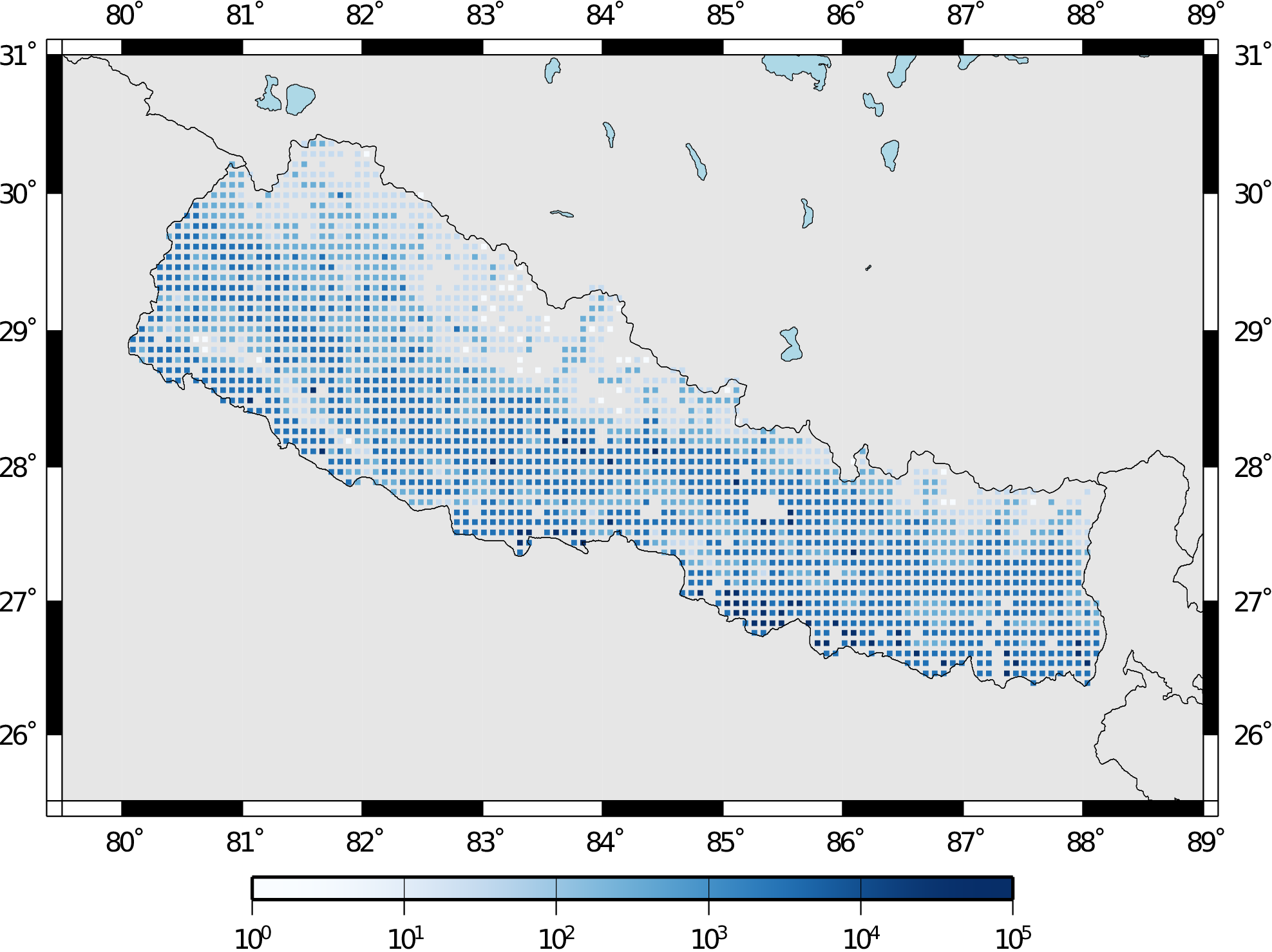
Fig. 3.12 Distribution of number of buildings in Nepal#
The building portfolio was organised into four classes for the rural areas (adobe, dressed stone, unreinforced fired brick, wooden frames), and five classes for the urban areas (the aforementioned typologies, in addition to reinforced concrete buildings). For each one of these building typologies, vulnerabilityfunctions and fragilityfunctions were collected from the published literature available for the region. These input models are only for demonstrative purposes and for further information about the building characteristics of Nepal, users are advised to contact the National Society for Earthquake Technology of Nepal (NSET - http:www.nset.org.np/).
The following sections include instructions not only on how to run the risk calculations, but also on how to produce the necessary hazard inputs. Thus, each demo comprises the configuration file, Exposure Model and fragility or vulnerability models fundamental for the risk calculations. Each demo folder also a configuration file and the input models to produce the relevant hazard inputs.
3.5.1. Scenario Damage#
Demos A rupture of magnitude Mw 7 in the central part of Nepal
is considered in this demo. The
characteristics of this rupture (geometry, dip, rake, hypocentre, upper
and lower seismogenic depth) are defined in the fault_rupture.xml
file, and the hazard and risk calculation settings are specified in the
job.ini file.
To run the Scenario Damage demo, users should navigate to the folder where the required files have been placed and employ following command:
user@ubuntu:~$ oq engine --run job_hazard.ini && oq engine --run job_risk.ini --hc=-1
The hazard calculation should produce the following outputs:
Calculation 8967 completed in 4 seconds. Results:
  id | name
9060 | Ground Motion Fields
9061 | Realizations
and the following outputs should be produced by the risk calculation:
Calculation 8968 completed in 16 seconds. Results:
  id | name
9062 | Average Asset Damages
9063 | Average Asset Losses
3.5.2. Scenario Risk Demos#
The same rupture described in the Scenario Damage demo is also used for this demo. In this case, a combined job file, job.ini, is used to specify the configuration parameters for the hazard and risk calculations.
To run the Scenario Risk demo, users should navigate to the folder where the required files have been placed and employ following command:
user@ubuntu:~$ oq engine --run job.ini
and the following outputs should be produced:
Calculation 8970 completed in 16 seconds. Results:
  id | name
9071 | Aggregate Asset Losses
9072 | Full Report
9073 | Ground Motion Fields
9074 | Average Asset Losses
9075 | Aggregate Event Losses
9076 | Realizations
3.5.3. Classical Probabilistic Seismic Damage Demos#
The seismic source model developed within the Global Seismic Hazard Assessment Program (GSHAP) is used with the (B. S.-J. Chiou and Youngs 2008) ground motion prediction equation to produce the hazard input for this demo. No uncertainties are considered in the seismic source model and since only one GMPE is being considered, there will be only one possible path in the logic tree. Therefore, only one set of seismic hazard curves will be produced. To run the hazard calculation, the following command needs to be employed:
user@ubuntu:~$ oq engine --run job_hazard.ini
which will produce the following sample hazard output:
Calculation 8971 completed in 34 seconds. Results:
  id | name
9074 | Hazard Curves
9075 | Realizations
The risk job calculates the probabilistic damage distribution for each asset in the Exposure Model starting from the above generated hazard curves. The following command launches the risk calculations:
user@ubuntu:~$ oq engine --run job_risk.ini --hc 8971
and the following sample outputs are obtained:
Calculation 8972 completed in 16 seconds. Results:
  id | name
9076 | Asset Damage Distribution
9077 | Asset Damage Statistics
3.5.4. Classical Probabilistic Seismic Risk Demos#
The same hazard input as described in the Classical Probabilistic Damage demo is used for this demo. Thus, the workflow to produce the set of hazard curves described in Section Classical Probabilistic Seismic Damage Demos is also valid herein. Then, to run the Classical Probabilistic Risk demo, users should navigate to the folder containing the demo input models and configuration files and employ the following command:
user@ubuntu:~$ oq engine --run job_hazard.ini
which will produce the following hazard output:
Calculation 8971 completed in 34 seconds. Results:
  id | name
9074 | Hazard Curves
9075 | Realizations
In this demo, loss exceedance curves for each asset and two probabilistic loss maps (for probabilities of exceedance of 1% and 10%) are produced. The following command launches these risk calculations:
user@ubuntu:~$ oq engine --run job_risk.ini --hc 8971
and the following outputs are expected:
Calculation 8973 completed in 16 seconds. Results:
  id | name
9077 | Asset Loss Curves Statistics
9078 | Asset Loss Maps Statistics
9079 | Average Asset Loss Statistics
3.5.5. Event Based Probabilistic Seismic Damage Demos#
This demo uses the same probabilistic seismic hazard assessment (PSHA) model described in the previous examples in Section Classical Probabilistic Seismic Damage Demos and Section Classical Probabilistic Seismic Risk Demos. However, instead of hazard curves, sets of ground motion fields will be generated by the hazard calculation of this demo. Again, since there is only one Branch in the logic tree, only one set of ground motion fields will be used in the risk calculations. The hazard and risk jobs are defined in a single configuration file for this demo. To trigger the hazard and risk calculations the following command needs to be used:
user@ubuntu:~$ oq engine --run job.ini
and the following results are expected:
Calculation 2 completed in 29 seconds. Results:
  id | name
  24 | Aggregate Event Damages
  30 | Aggregate Event Losses
  20 | Average Asset Damages
  21 | Average Asset Damages Statistics
  22 | Average Asset Losses
  23 | Average Asset Losses Statistics
  32 | Earthquake Ruptures
  25 | Events
  26 | Full Report
  27 | Ground Motion Fields
  28 | Hazard Curves
  29 | Input Files
  31 | Realizations
3.5.6. Event Based Probabilistic Seismic Risk Demos#
This demo uses the same probabilistic seismic hazard assessment (PSHA) model described in the previous examples in Section Classical Probabilistic Seismic Damage Demos and Section Classical Probabilistic Seismic Risk Demos. However, instead of hazard curves, sets of ground motion fields will be generated by the hazard calculation of this demo. Again, since there is only one Branch in the logic tree, only one set of ground motion fields will be used in the risk calculations. The hazard and risk jobs are defined in a single configuration file for this demo. To trigger the hazard and risk calculations the following command needs to be used:
user@ubuntu:~$ oq engine --run job.ini
and the following results are expected:
Calculation 8974 completed in 229 seconds. Results:
  id | name
1820 | Total Loss Curves
1821 | Total Loss Curves Statistics
1822 | Aggregate Loss Table
1823 | Average Asset Losses
1824 | Average Asset Loss Statistics
1826 | Asset Loss Maps
1827 | Asset Loss Maps Statistics
1828 | Average Asset Losses
1829 | Average Asset Losses Statistics
1830 | Earthquake Ruptures
1831 | Events
1832 | Realizations
The number and the name of the outputs can change between different versions of the engine.
3.5.7. Retrofit Benefit-Cost Ratio Demos#
The loss exceedance curves used within this demo are produced using the Classical Probabilistic Risk calculator. Thus, the process to produce the seismic hazard curves described in Section Classical Probabilistic Seismic Risk Demos can be employed here. Then, the risk calculations can be initiated using the following command:
user@ubuntu:~$ oq engine --run job_risk.ini --hc 8971
which should produce the following output:
Calculation 8976 completed in 14 seconds. Results:
  id | name
9087 | Benefit Cost Ratios
3.6. Bibliography#
Aki, K., and P. G. Richards. 2002. Quantitative Seismology. Sausalito, California: University Science Books.
Chiou, B. S.-J., and R. R. Youngs. 2008. “An NGA Model for the Average Horizontal Component of Peak Ground Motion and Response Spectra.” Earthquake Spectra 24: 173–215.
Chiou, Brian S.-J., and Robert R. Youngs. 2014. “Update of the Chiou and Youngs NGA Model for the Average Horizontal Component of Peak Ground Motion and Response Spectra.” Earthquake Spectra 30 (3): 1117–53.
Cornell, C. A. 1968. “Engineering Seismic Risk Analysis.” Bulletin of the Seismological Society of America 58: 1583–1606.
EPRI, Electric Power Research Institute. 2011. “Technical Report: Central and Eastern United States Seismic Source Characterisation for Nuclear Facilities.” Report. EPRI, Palo Alto, CA. U. S. DoE,; U. S. NERC.
Field, E. H., T. H. Jordan, and C. A. Cornell. 2003. “OpenSHA - a Developing Community-Modeling Environment for Seismic Hazard Analysis.” Seismological Research Letters 74: 406–19.
Frankel, A. 1995. “Mapping Seismic Hazard in the Central and Eastern United States.” Seismological Research Letters 66 (4): 8–21.
McGuire, K. K. 1976. “FORTRAN Computer Program for Seismic Risk Analysis.” Open-File report 76-67. United States Department of the Interior, Geological Survey.
Petersen, M. D., A. D. Frankel, S. C. Harmsen, C. S. Mueller, K. M. Haller, R. L. Wheeler, R. L. Wesson, et al. 2008. “Documentation for the 2008 Update of the United States National Seismic Hazard Maps.” Open File Report 2008-1128. U.S. Department of the Interior, U.S. Geological Survey.
Schwartz, D. P., and K. J. Coppersmith. 1984. “Fault Behaviour and Characteristic Earthquakes: Examples from the Wasatch and San Andreas Fault Zones.” Journal of Geophysical Research 89 (B7): 5681–98.
Strasser, F. O., M. C. Arango, and J. J. Bommer. 2010. “Scaling of the Source Dimensions of Interface and Intraslab Subduction-zone Earthquakes with Moment Magnitude.” Seismological Research Letters 81: 941–50.
Thingbaijam, K. K. S., P. M. Mai, and K. Goda. 2017. “New Empirical Earthquake Source-Scaling Laws.” Bulletin of the Seismological Society of America 107 (5): 2225–2946. https://doi.org/10.1785/0120170017.
Wells, D. L., and K. J. Coppersmith. 1994. “New Empirical Relationships Among Magnitude, Rupture Length, Rupture Width, Rupture Area, and Surface Displacement.” Bulletin of the Seismological Society of America 84 (4): 974–1002.
Woo, G. 1996. “Kernel Estimation Methods for Seismic Hazard Area Source Modeling.” Bulletin of the Seismological Society of America 86 (2): 353–62.
Youngs, R. R., and K. J. Coppersmith. 1985. “Implications of Fault Slip Rates and Earthquake Recurrence Models to Probabilistic Seismic Hazard Estimates.” Bulletin of the Seismological Society of America 75 (April): 939–64.
- 2
Within the OpenQuake engine, longitude and latitude coordinates are internally rounded to a precision of 5 digits after the decimal point.
- 3
Note that as of OpenQuake engine18, the uncertainty in the consequence ratios is ignored, and only the mean consequence ratios for the set of limit states is considered when computing the consequences from the damage distribution. Consideration of the uncertainty in the consequence ratios is planned for future releases of the OpenQuake engine.
- 4
As of OpenQuake engine18, the “PM” option for defining vulnerabilityfunctions is supported by the Scenario Risk and the Stochastic Event-Based Probabilistic Risk Calculators, but not by the Classical Probabilistic Risk Calculator.