2. Hazard#
2.1. Introduction to the Hazard Module#
The hazard component of the OpenQuake engine builds on top of the OpenQuake hazard library (oq-hazardlib), a Python-based library containing tools for PSHA calculations.
In this section we briefly illustrate the main properties of the hazard component of the OpenQuake engine. In particular, we will describe the main typologies of sources supported and the main calculation workflows available.
2.1.1. Source typologies#
An OpenQuake engine seismic source input model contains a list of sources belonging to a finite set of possible typologies. Each source type is defined by a set of parameters - called source data - which are used to specify the source geometry and the properties of seismicity occurrence.
Currently the OpenQuake engine supports the following source types:
Sources for modelling distributed seismicity:
Point Source - The elemental source type used to model distributed seismicity. Grid and area sources (described below) are different containers of point sources.
Area Source - So far, the most frequently adopted source type in national and regional PSHA models.
Grid Source - A replacement for area sources admitting spatially variable seismicity occurrence properties.
Fault sources with floating ruptures:
Simple Fault Source - The simplest fault model in the OpenQuake engine. This source is habitually used to describe shallow seismogenic faults.
Complex Fault Source - Often used to model subduction interface sources with a complex geometry.
Fault sources with ruptures always covering the entire fault surface:
Characteristic Fault Source - A typology of source where ruptures always fill the entire fault surface.
Non-Parametric Source - A typology of source representing a collection of ruptures, each with their associated probabilities of 0, 1, 2 … occurrences in the investigation time
Sources for representing individual earthquake ruptures
Planar fault rupture - an individual fault rupture represented as a single rectangular plane
Multi-planar fault rupture - an individual rupture represented as a collection of rectangular planes
Simple fault rupture - an individual fault rupture represented as a simple fault surface
Complex fault rupture - an individual fault rupture represented as a complex fault surface
The OpenQuake engine contains some basic assumptions for the definition of these source typologies:
In the case of area and fault sources, the seismicity is homogeneously distributed over the source;
Seismicity temporal occurrence follows a Poissonian model.
The above sets of sources may be referred to as “parametric” sources, that is to say that the generation of the Earthquake Rupture Forecast is done by the OpenQuake engine based on the parameters of the sources set by the user. In some cases, particularly if the user wishes for the temporal occurrence model to be non-Poissonian (such as the lognormal or Brownian Passage Time models) a different type of behaviour is needed. For this OpenQuake-engine supports a Non-Parametric Source in which the Earthquake Rupture Forecast is provided explicitly by the user as a set of ruptures and their corresponding probabilities of occurrence.
2.1.1.1. Source typologies for modelling distributed seismicity#
2.1.1.1.1. Point sources#
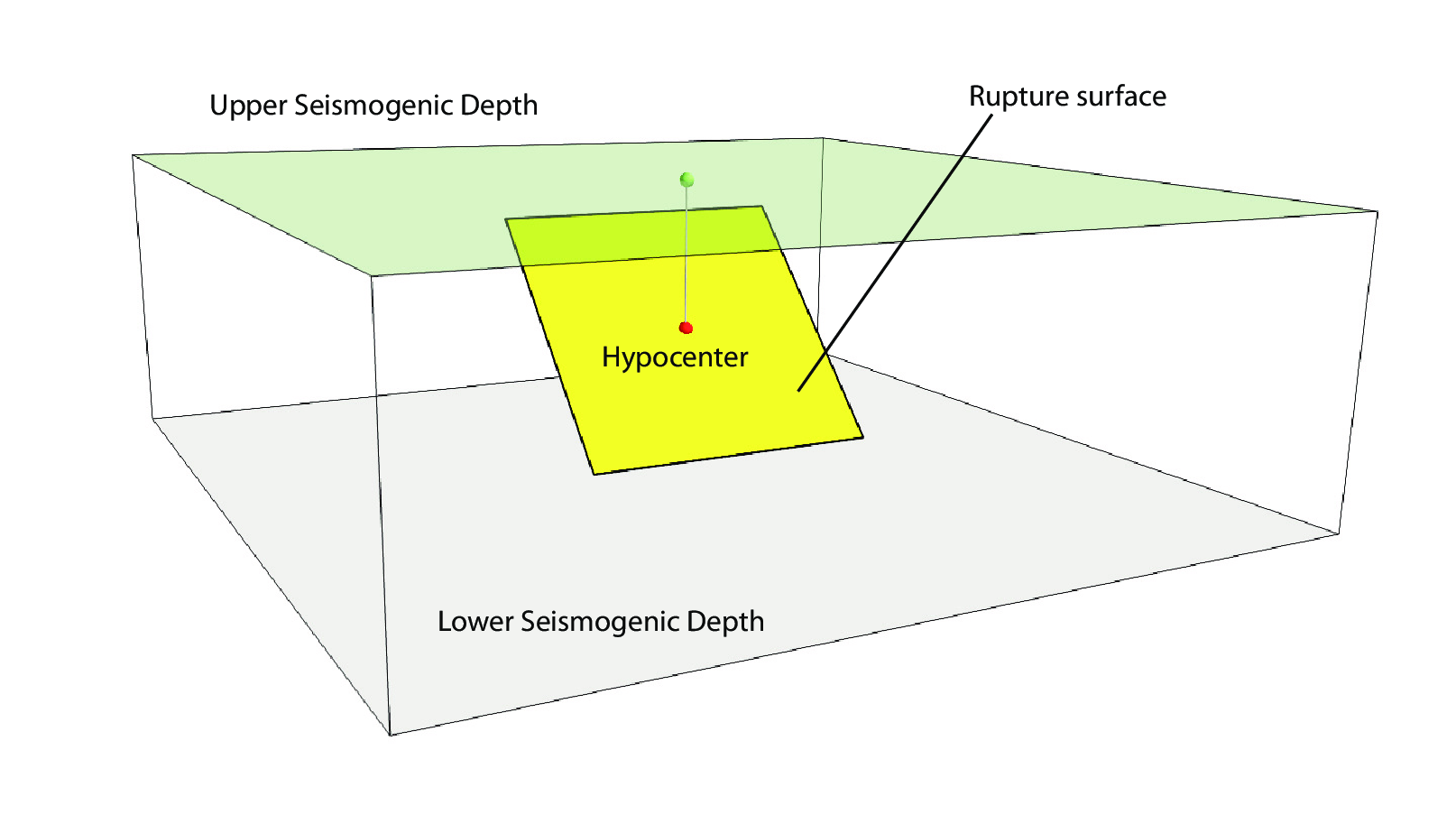
Fig. 2.1 Single rupture#
The point source is the elemental source type adopted in the OpenQuake-engine for modelling distributed seismicity. The OpenQuake engine always performs calculations considering finite ruptures, even in the case of point sources.
These are the basic assumptions used to generate ruptures with point sources:
Ruptures have a rectangular shape
Rupture hypocenter is located in the middle of the rupture
Ruptures are limited at the top and at the bottom by two planes parallel to the sea level and placed at two characteristic depths named upper and lower seismogenic depths, respectively (see Fig. 2.1)
2.1.1.1.1.1. Source data#
For the definition of a point source the following parameters are required (Fig. 2.1 shows some of the parameters described below, together with an example of the surface of a generated rupture):
The coordinates of the point (i.e. longitude and latitude) [decimal degrees]
The upper and lower seismogenic depths [km]
One Magnitude-Frequency Distribution
One magnitude-scaling relationship
The rupture aspect ratio
A distribution of nodal planes i.e. one (or several) instances of the following set of parameters:
strike [degrees]
dip [degrees]
rake [degrees]
A magnitude independent depth distribution of hypocenters [km].
Fig. 2.2 shows ruptures generated by a point source for a range of magnitudes. Each rupture is centered on the single hypocentral position admitted by this point source. Ruptures are created by conserving the area computed using the specified magnitude-area scaling relatioship and the corresponding value of magnitude.
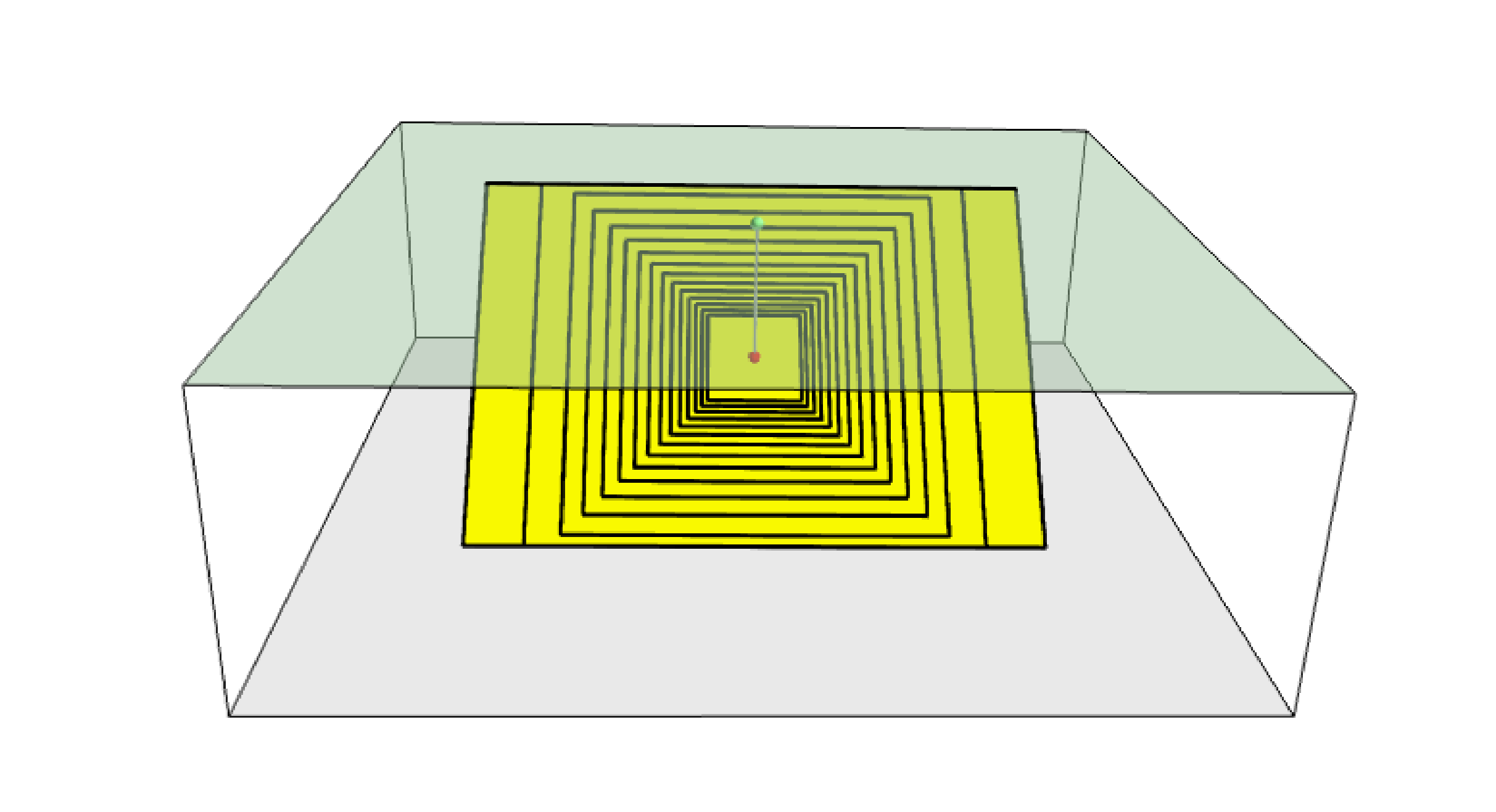
Fig. 2.2 Point source with multiple ruptures. Note the change in the aspect ratio once the rupture width fills the entire seismogenic layer.#
Below we provide the excerpt of an .xml file used to describe the properties of a point source. Note that in this example, ruptures occur on two possible nodal planes and two hypocentral depths. Fig. 2.3 shows the ruptures generated by the point source.
 1<pointSource id="1" name="point" tectonicRegion="Stable Continental Crust">
 2     <pointGeometry>
 3         <gml:Point>
 4             <gml:pos>-122.0 38.0</gml:pos>
 5         </gml:Point>
 6         <upperSeismoDepth>0.0</upperSeismoDepth>
 7         <lowerSeismoDepth>10.0</lowerSeismoDepth>
 8    </pointGeometry>
 9    <magScaleRel>WC1994</magScaleRel>
10    <ruptAspectRatio>0.5</ruptAspectRatio>
11    <truncGutenbergRichterMFD aValue="-3.5" bValue="1.0" minMag="5.0"
12                                maxMag="6.5" />
13    <nodalPlaneDist>
14         <nodalPlane probability="0.3" strike="0.0" dip="90.0" rake="0.0" />
15         <nodalPlane probability="0.7" strike="90.0" dip="45.0" rake="90.0" />
16    </nodalPlaneDist>
17    <hypoDepthDist>
18        <hypoDepth probability="0.5" depth="4.0" />
19        <hypoDepth probability="0.5" depth="8.0" />
20    </hypoDepthDist>
21</pointSource>

Fig. 2.3 Ruptures produced by the source created using the information in the example .xml file described on page .#
2.1.1.1.2. Grid sources#
A Grid Source is simply a collection of point sources distributed over a regular grid (usually equally spaced in longitude and latitude). In Probabilistic Seismic Hazard Analysis a grid source can be considered a model alternative to area sources, since they both model distributed seismicity. Grid sources are generally used to reproduce more faithfully the spatial pattern of seismicity depicted by the earthquakes occurred in the past; in some models (e.g. Petersen et al. (2008)) only events of low and intermediate magnitudes are considered. They are frequently, though not always, computed using seismicity smoothing algorithms (Frankel 1995; Woo 1996, amongst many others).
The use of smoothing algorithms to produce grid sources brings some advantages compared to area sources, since (1) it removes most of the unavoidable degree of subjectivity due to the definition of the geometries of the area sources and (2) it produces a spatial pattern of seismicity that is usually closer to what observed in the reality. Nevertheless, in many cases smoothing algorithms require an a-priori definition of some setup parameters that expose the calculation to a certain degree of partiality.
Grid sources are modeled in OpenQuake engine simply as a set of point sources; in other words, a grid source is just a long list of point sources specified as described in the previous section.
2.1.1.1.3. Area sources#
Area sources are usually adopted to describe the seismicity occurring over wide areas where the identification and characterization - i.e. the unambiguous definition of position, geometry and seismicity occurrence parameters - of single fault structures is difficult.
From a computation standpoint, area sources are comparable to grid sources since they are both represented in the engine by a list of point sources.
The OpenQuake engine using the source data parameters (see below) creates an equally spaced in distance grid of point sources where each point has the same seismicity occurrence properties (i.e. rate of events generated).
Below we provide a brief description of the parameters necessary to completely describe an area source.
2.1.1.1.3.1. Source data#
A polygon defining the external border of the area (i.e. a list of Longitude-Latitude [degrees] tuples) The current version of the OQ-engine doesn’t support the definition of internal borders.
The upper and lower seismogenic depths [km]
One Magnitude-Frequency Distribution
One Magnitude-Scaling Relationship
The rupture aspect ratio
A distribution of nodal planes i.e. one (or several) instances of the following set of parameters
strike [degrees]
dip [degrees]
rake [degrees]
A magnitude independent depth distribution of hypocenters [km].
Below we provide the excerpt of an .xml file used to describe the properties of an area source. The ruptures generated by the area source described in the example are controlled by two nodal planes and have hypocenters at localized at two distinct depths.
 1<areaSource id="1" name="Quito" tectonicRegion="Active Shallow Crust">
 2    <areaGeometry>
 3      <gml:Polygon>
 4        <gml:exterior>
 5          <gml:LinearRing>
 6            <gml:posList>
 7              -122.5 37.5
 8              -121.5 37.5
 9              -121.5 38.5
10              -122.5 38.5
11            </gml:posList>
12          </gml:LinearRing>
13        </gml:exterior>
14      </gml:Polygon>
15      <upperSeismoDepth>0.0</upperSeismoDepth>
16      <lowerSeismoDepth>10.0</lowerSeismoDepth>
17    </areaGeometry>
18    <magScaleRel>PeerMSR</magScaleRel>
19    <ruptAspectRatio>1.5</ruptAspectRatio>
20    <incrementalMFD minMag="6.55" binWidth="0.1">
21        <occurRates>0.0010614989 8.8291627E-4 7.3437777E-4 6.108288E-4
22                    5.080653E-4</occurRates>
23    </incrementalMFD>
24    <nodalPlaneDist>
25        <nodalPlane probability="0.3" strike="0.0" dip="90.0" rake="0.0"/>
26        <nodalPlane probability="0.7" strike="90.0" dip="45.0" rake="90.0"/>
27    </nodalPlaneDist>
28    <hypoDepthDist>
29        <hypoDepth probability="0.5" depth="4.0" />
30        <hypoDepth probability="0.5" depth="8.0" />
31    </hypoDepthDist>
32</areaSource>
2.1.1.2. Fault sources with floating ruptures#
Fault sources in the OpenQuake engine are classified according to the method adopted to distribute ruptures over the fault surface. Two options are currently supported:
With the first option, ruptures with a surface lower than the whole fault surface are floated so as to cover as much as possible homogeneously the fault surface. This model is compatible with all the supported magnitude-frequency distributions.
With the second option, ruptures always fill the entire fault surface. This model is compatible with magnitude-frequency distributions similar to a characteristic model (à la (Schwartz and Coppersmith 1984)).
In this subsection we discuss the different fault source types that support floating ruptures. In the next subsection we will illustrate the fault typology available to model a characteristic rupturing behaviour.
2.1.1.2.1. Simple Faults#
Simple Faults are the most common source type used to model shallow faults; the “simple” adjective relates to the geometry description of the source which is obtained by projecting the fault trace (i.e. a polyline) along a characteristic dip direction.
The parameters used to create an instance of this source type are described in the following paragraph.
2.1.1.2.1.1. Source data#
A horizontal Fault Trace (usually a polyline). It is a list of longitude-latitude tuples [degrees].
A Frequency-Magnitude Distribution
A Magnitude-Scaling Relationship
A representative value of the dip angle (specified following the Aki-Richards convention; see Aki and Richards (2002)) [degrees]
Rake angle (specified following the Aki-Richards convention; see Aki and Richards (2002)) [degrees]
Upper and lower depth values limiting the seismogenic interval [km]
For near-fault probabilistic seismic hazard analysis, two additional parameters are needed for characterising seismic sources:
A hypocentre list. It is a list of the possible hypocentral positions, and the corresponding weights, e.g., alongStrike=”0.25” downDip=”0.25” weight=”0.25”. Each hypocentral position is defined in relative terms using as a reference the upper left corner of the rupture and by specifying the fraction of rupture length and rupture width.
A slip list. It is a list of the possible rupture slip directions [degrees], and their corresponding weights. The angle describing each slip direction is measured counterclockwise using the fault strike direction as reference.
In near-fault PSHA calculations, the hypocentre list and the slip list
are mandatory. The weights in each list must always sum to one. The
available GMPE which currently supports the near-fault directivity PSHA
calculation in OQ- engine is the ChiouYoungs2014NearFaultEffect GMPE
developed by Brian S.-J. Chiou and Youngs (2014) (associated with an
Active Shallow Crust tectonic region type).
We provide two examples of simple fault source files. The first is an excerpt of an xml file used to describe the properties of a simple fault source and the second example shows the excerpt of an xml file used to describe the properties of a simple fault source that can be used to perform a PSHA calculation taking into account directivity effects.
 1<simpleFaultSource id="1" name="Mount Diablo Thrust"
 2        tectonicRegion="Active Shallow Crust">
 3      <simpleFaultGeometry>
 4          <gml:LineString>
 5              <gml:posList>
 6                  -121.82290 37.73010
 7                  -122.03880 37.87710
 8              </gml:posList>
 9          </gml:LineString>
10          <dip>45.0</dip>
11          <upperSeismoDepth>10.0</upperSeismoDepth>
12          <lowerSeismoDepth>20.0</lowerSeismoDepth>
13      </simpleFaultGeometry>
14      <magScaleRel>WC1994</magScaleRel>
15      <ruptAspectRatio>1.5</ruptAspectRatio>
16      <incrementalMFD minMag="5.0" binWidth="0.1">
17          <occurRates>0.0010614989 8.8291627E-4 7.3437777E-4 6.108288E-4
18                      5.080653E-4</occurRates>
19      </incrementalMFD>
20      <rake>30.0</rake>
21      <hypoList>
22          <hypo alongStrike="0.25" downDip="0.25" weight="0.25"/>
23          <hypo alongStrike="0.25" downDip="0.75" weight="0.25"/>
24          <hypo alongStrike="0.75" downDip="0.25" weight="0.25"/>
25          <hypo alongStrike="0.75" downDip="0.75" weight="0.25"/>
26      </hypoList>
27      <slipList>
28          <slip weight="0.333">0.0</slip>
29          <slip weight="0.333">45.0</slip>
30          <slip weight="0.334">90.0</slip>
31      </slipList>
32</simpleFaultSource>
 1<simpleFaultSource id="1" name="Mount Diablo Thrust"
 2        tectonicRegion="Active Shallow Crust">
 3     <simpleFaultGeometry>
 4         <gml:LineString>
 5             <gml:posList>
 6                 -121.82290 37.73010
 7                 -122.03880 37.87710
 8             </gml:posList>
 9         </gml:LineString>
10         <dip>45.0</dip>
11         <upperSeismoDepth>10.0</upperSeismoDepth>
12         <lowerSeismoDepth>20.0</lowerSeismoDepth>
13     </simpleFaultGeometry>
14     <magScaleRel>WC1994</magScaleRel>
15     <ruptAspectRatio>1.5</ruptAspectRatio>
16     <incrementalMFD minMag="5.0" binWidth="0.1">
17         <occurRates>0.0010614989 8.8291627E-4 7.3437777E-4 6.108288E-4
18                     5.080653E-4</occurRates>
19     </incrementalMFD>
20     <rake>30.0</rake>
21     <hypoList>
22         <hypo alongStrike="0.25" downDip="0.25" weight="0.25"/>
23         <hypo alongStrike="0.25" downDip="0.75" weight="0.25"/>
24         <hypo alongStrike="0.75" downDip="0.25" weight="0.25"/>
25         <hypo alongStrike="0.75" downDip="0.75" weight="0.25"/>
26     </hypoList>
27     <slipList>
28         <slip weight="0.333">0.0</slip>
29         <slip weight="0.333">45.0</slip>
30         <slip weight="0.334">90.0</slip>
31     </slipList>
32</simpleFaultSource>
2.1.1.2.2. Complex Faults#
A complex fault differs from simple fault just by the way the geometry of the fault surface is defined and the fault surface is later created. The input parameters used to describe complex faults are, for the most part, the same used to describe the simple fault typology.
In the case of complex faults, the dip angle is not requested while the fault trace is substituted by two fault edges limiting the top and bottom of the fault surface. Additional curves lying over the fault surface can be specified to complement and refine the description of the fault surface geometry. Unlike the simple fault these edges are not required to be horizontal and may vary in elevation, i.e. the upper edge may represent the intersection between the exposed fault trace and the topographic surface, where positive values indicate below sea level, and negative values indicate above sea level.
Usually, we use complex faults to model intraplate megathrust faults such as the big subduction structures active in the Pacific (Sumatra, South America, Japan) but this source typology can be used also to create - for example - listric fault sources with a realistic geometry.
 1<complexFaultSource id="1" name="Cascadia Megathrust"
 2                    tectonicRegion="Subduction Interface">
 3    <complexFaultGeometry>
 4        <faultTopEdge>
 5            <gml:LineString>
 6                <gml:posList>
 7                    -124.704  40.363  0.5493260E+01
 8                    -124.977  41.214  0.4988560E+01
 9                    -125.140  42.096  0.4897340E+01
10                </gml:posList>
11            </gml:LineString>
12        </faultTopEdge>
13        <intermediateEdge>
14            <gml:LineString>
15                <gml:posList>
16                    -124.704  40.363  0.5593260E+01
17                    -124.977  41.214  0.5088560E+01
18                    -125.140  42.096  0.4997340E+01
19                </gml:posList>
20            </gml:LineString>
21        </intermediateEdge>
22        <intermediateEdge>
23            <gml:LineString>
24                <gml:posList>
25                    -124.704  40.363  0.5693260E+01
26                    -124.977  41.214  0.5188560E+01
27                    -125.140  42.096  0.5097340E+01
28                </gml:posList>
29            </gml:LineString>
30        </intermediateEdge>
31        <faultBottomEdge>
32            <gml:LineString>
33                <gml:posList>
34                    -123.829  40.347  0.2038490E+02
35                    -124.137  41.218  0.1741390E+02
36                    -124.252  42.115  0.1752740E+02
37                </gml:posList>
38            </gml:LineString>
39        </faultBottomEdge>
40    </complexFaultGeometry>
41    <magScaleRel>WC1994</magScaleRel>
42    <ruptAspectRatio>1.5</ruptAspectRatio>
43    <truncGutenbergRichterMFD aValue="-3.5" bValue="1.0" minMag="5.0"
44                              maxMag="6.5" />
45    <rake>30.0</rake>
46</complexFaultSource>
As with the previous examples, the red text highlights the parameters used to specify the source geometry, the parameters in green describe the rupture mechanism, the text in blue describes the magnitude-frequency distribution and the gray text describes the rupture properties.
2.1.1.3. Fault sources without floating ruptures#
2.1.1.3.1. Characteristic faults#
The characteristic fault source is a particular typology of fault created with the assumption that its ruptures will always cover the entire fault surface. As such, no floating is necessary on the surface. The characteristic fault may still take as input a magnitude frequency distribution. In this case, the fault surface can be represented either as a Simple Fault Source surface or as a Complex Fault Source surface or as a combination of rectangular ruptures as represented in Fig. 2.4. Mutiple surfaces containing mixed geometry types are also supported.
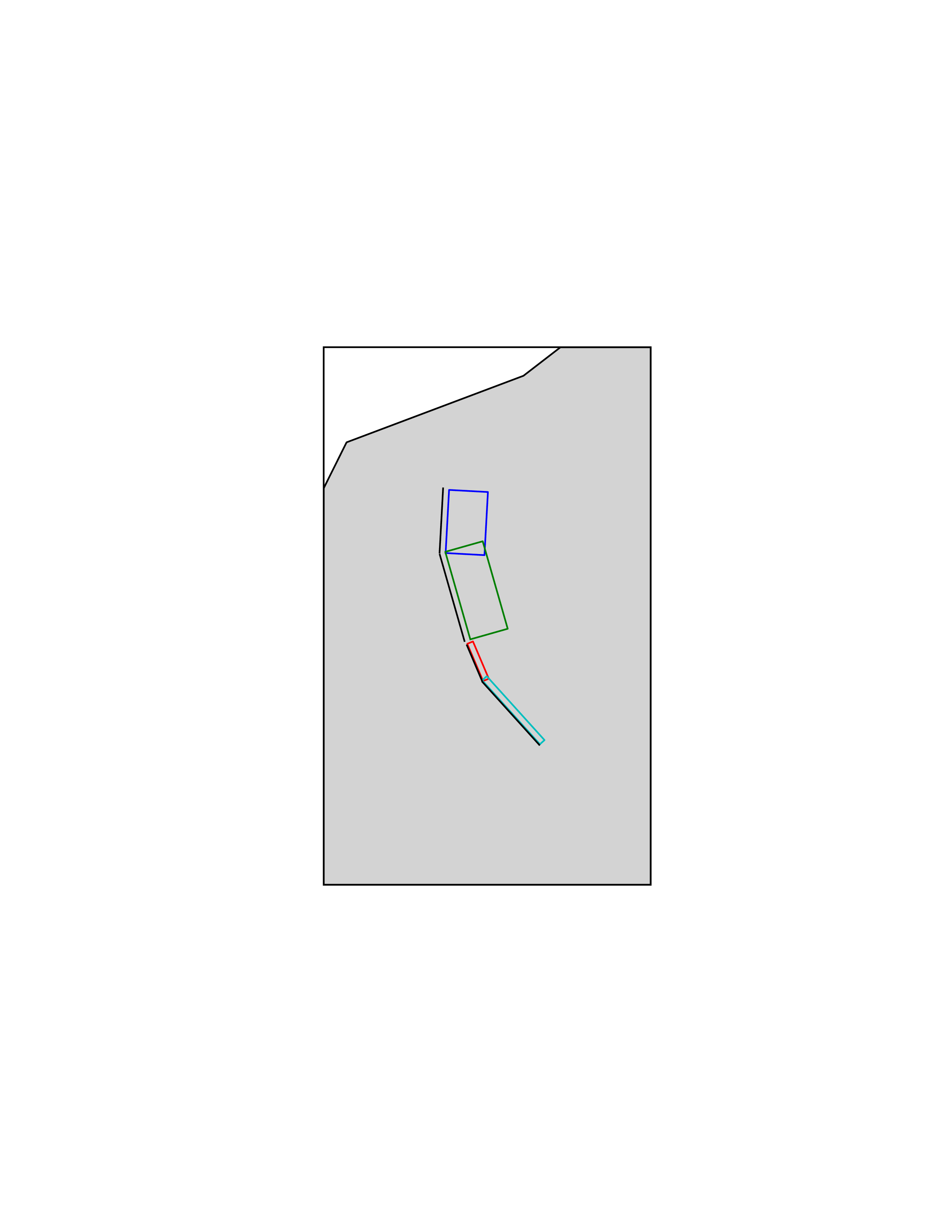
Fig. 2.4 Geometry of a multi-segmented characteristic fault composed of four rectangular ruptures as modelled in OpenQuake.#
2.1.1.3.1.1. Source data#
The characteristic rupture surface is defined through one of the following options:
A list of rectangular ruptures (“planar surfaces”)
A Simple Fault Source geometry
A Complex Fault Source geometry
A Frequency-Magnitude Distribution.
Rake angle (specified following the Aki-Richards convention; see Aki and Richards (2002)).
Upper and lower depth values limiting the seismogenic interval.
A comprehensive example enumerating the possible rupture surface configurations is shown below.
 1<characteristicFaultSource id="5" name="characteristic source, simple fault"
 2                           tectonicRegion="Volcanic">
 3    <truncGutenbergRichterMFD aValue="-3.5" bValue="1.0"
 4                              minMag="5.0" maxMag="6.5" />
 5    <rake>30.0</rake>
 6    <surface>
 7        <!-- Characteristic Fault with a simple fault surface -->
 8        <simpleFaultGeometry>
 9            <gml:LineString>
10                <gml:posList>
11                    -121.82290 37.73010
12                    -122.03880 37.87710
13                </gml:posList>
14            </gml:LineString>
15            <dip>45.0</dip>
16            <upperSeismoDepth>10.0</upperSeismoDepth>
17            <lowerSeismoDepth>20.0</lowerSeismoDepth>
18        </simpleFaultGeometry>
19    </surface>
20</characteristicFaultSource>
 1<characteristicFaultSource id="6" name="characteristic source, complex fault"
 2                           tectonicRegion="Volcanic">
 3    <incrementalMFD minMag="5.0" binWidth="0.1">
 4        <occurRates>0.0010614989 8.8291627E-4 7.3437777E-4</occurRates>
 5    </incrementalMFD>
 6    <rake>60.0</rake>
 7    <surface>
 8        <!-- Characteristic source with a complex fault surface -->
 9        <complexFaultGeometry>
10            <faultTopEdge>
11                <gml:LineString>
12                    <gml:posList>
13                       -124.704  40.363  0.5493260E+01
14                       -124.977  41.214  0.4988560E+01
15                       -125.140  42.096  0.4897340E+01
16                    </gml:posList>
17                </gml:LineString>
18            </faultTopEdge>
19            <faultBottomEdge>
20                <gml:LineString>
21                    <gml:posList>
22                        -123.829  40.347  0.2038490E+02
23                        -124.137  41.218  0.1741390E+02
24                        -124.252  42.115  0.1752740E+02
25                    </gml:posList>
26                </gml:LineString>
27            </faultBottomEdge>
28        </complexFaultGeometry>
29    </surface>
30</characteristicFaultSource>
 1<characteristicFaultSource id="7" name="characteristic source, multi surface"
 2                           tectonicRegion="Volcanic">
 3    <truncGutenbergRichterMFD aValue="-3.6" bValue="1.0"
 4                              minMag="5.2" maxMag="6.4" />
 5    <rake>90.0</rake>
 6    <surface>
 7        <!-- Characteristic source with a collection of planar surfaces -->
 8        <planarSurface>
 9            <topLeft lon="-1.0" lat="1.0" depth="21.0" />
10            <topRight lon="1.0" lat="1.0" depth="21.0" />
11            <bottomLeft lon="-1.0" lat="-1.0" depth="59.0" />
12            <bottomRight lon="1.0" lat="-1.0" depth="59.0" />
13        </planarSurface>
14        <planarSurface strike="20.0" dip="45.0">
15             <topLeft lon="1.0" lat="1.0" depth="20.0" />
16             <topRight lon="3.0" lat="1.0" depth="20.0" />
17             <bottomLeft lon="1.0" lat="-1.0" depth="80.0" />
18             <bottomRight lon="3.0" lat="-1.0" depth="80.0" />
19         </planarSurface>
20    </surface>
21</characteristicFaultSource>
2.1.1.4. Non-Parametric Sources#
2.1.1.4.1. Non-Parametric Fault#
The non-parametric fault typology requires that the user indicates the rupture properties (rupture surface, magnitude, rake and hypocentre) and the corresponding probabilities of the rupture. The probabilities are given as a list of floating point values that correspond to the probabilities of \(0, 1, 2, \ldots ... N\) occurrences of the rupture within the specified investigation time. Note that there is not, at present, any internal check to ensure that the investigation time to which the probabilities refer corresponds to that specified in the configuration file. As the surface of the rupture is set explicitly, no rupture floating occurs, and, as in the case of the characteristic fault source, the rupture surface can be defined as either a single planar rupture, a list of planar ruptures, a Simple Fault Source geometry, a Complex Fault Source geometry, or a combination of different geometries.
Comprehensive examples enumerating the possible configurations are shown below:
 1<nonParametricSeismicSource id="1" name="A Non Parametric Planar Source"
 2                            tectonicRegion="Some TRT">
 3    <singlePlaneRupture probs_occur="0.544 0.456">
 4        <magnitude>8.3</magnitude>
 5        <rake>90.0</rake>
 6        <hypocenter depth="26.101" lat="40.726" lon="143.0"/>
 7        <planarSurface>
 8            <topLeft depth="9.0" lat="41.6" lon="143.1"/>
 9            <topRight depth="9.0" lat="40.2" lon="143.91"/>
10            <bottomLeft depth="43.202" lat="41.252" lon="142.07"/>
11            <bottomRight depth="43.202" lat="39.852" lon="142.91"/>
12        </planarSurface>
13    </singlePlaneRupture>
14    <multiPlanesRupture probs_occur="0.9244 0.0756">
15        <magnitude>6.9</magnitude>
16        <rake>0.0</rake>
17        <hypocenter depth="7.1423" lat="35.296" lon="139.31"/>
18        <planarSurface>
19            <topLeft depth="2.0" lat="35.363" lon="139.16"/>
20            <topRight depth="2.0" lat="35.394" lon="138.99"/>
21            <bottomLeft depth="14.728" lat="35.475" lon="139.19"/>
22            <bottomRight depth="14.728" lat="35.505" lon="139.02"/>
23        </planarSurface>
24        <planarSurface>
25            <topLeft depth="2.0" lat="35.169" lon="139.34"/>
26            <topRight depth="2.0" lat="35.358" lon="139.17"/>
27            <bottomLeft depth="12.285" lat="35.234" lon="139.45"/>
28            <bottomRight depth="12.285" lat="35.423" lon="139.28"/>
29        </planarSurface>
30    </multiPlanesRupture>
31</nonParametricSeismicSource>
 1<nonParametricSeismicSource id="2" name="A Non Parametric (Simple) Source"
 2                            tectonicRegion="Some TRT">
 3    <simpleFaultRupture probs_occur="0.157 0.843">
 4        <magnitude>7.8</magnitude>
 5        <rake>90.0</rake>
 6        <hypocenter depth="22.341" lat="43.624" lon="147.94"/>
 7        <simpleFaultGeometry>
 8            <gml:LineString>
 9                <gml:posList>
10                    147.96 43.202
11                    148.38 43.438
12                    148.51 43.507
13                    148.68 43.603
14                    148.76 43.640
15                </gml:posList>
16            </gml:LineString>
17            <dip>30.0</dip>
18            <upperSeismoDepth>14.5</upperSeismoDepth>
19            <lowerSeismoDepth>35.5</lowerSeismoDepth>
20        </simpleFaultGeometry>
21    </simpleFaultRupture>
22</nonParametricSeismicSource>
 1<nonParametricSeismicSource id="3" name="A Non Parametric (Complex) Source"
 2                            tectonicRegion="Some TRT">
 3    <complexFaultRupture probs_occur="0.157 0.843">
 4        <magnitude>7.8</magnitude>
 5        <rake>90.0</rake>
 6        <hypocenter depth="22.341" lat="43.624" lon="147.94"/>
 7        <complexFaultGeometry>
 8            <faultTopEdge>
 9                <gml:LineString>
10                    <gml:posList>
11                        148.76 43.64 5.0
12                        148.68 43.603 5.0
13                        148.51 43.507 5.0
14                        148.38 43.438 5.0
15                        147.96 43.202 5.0
16                    </gml:posList>
17                </gml:LineString>
18            </faultTopEdge>
19            <faultBottomEdge>
20               <gml:LineString>
21                    <gml:posList>
22                        147.92 44.002 35.5
23                        147.81 43.946 35.5
24                        147.71 43.897 35.5
25                        147.5 43.803 35.5
26                        147.36 43.727 35.5
27                    </gml:posList>
28                </gml:LineString>
29            </faultBottomEdge>
30        </complexFaultGeometry>
31    </complexFaultRupture>
32</nonParametricSeismicSource>
2.1.2. Magnitude-frequency distributions#
The magnitude-frequency distributions currently supported by the OpenQuake engine are the following:
- A discrete incremental magnitude-frequency distribution
It is the simplest distribution supported. It is defined by the minimum value of magnitude (representing the mid point of the first bin) and the bin width. The distribution itself is simply a sequence of floats describing the annual number of events for different bins. The maximum magnitude admitted by this magnitude-frequency distribution is just the sum of the minimum magnitude and the product of the bin width by the number annual rate values. Below we provide an example of the xml that should be incorporated in a seismic source description in order to define this Magnitude-Frequency Distribution.
1<incrementalMFD minMag="5.05" binWidth="0.1">
2    <occurRates>0.15 0.08 0.05 0.03 0.015</occurRates>
3</incrementalMFD>
The magnitude-frequency distribution obtained with the above parameters is represented in Fig. 2.5.
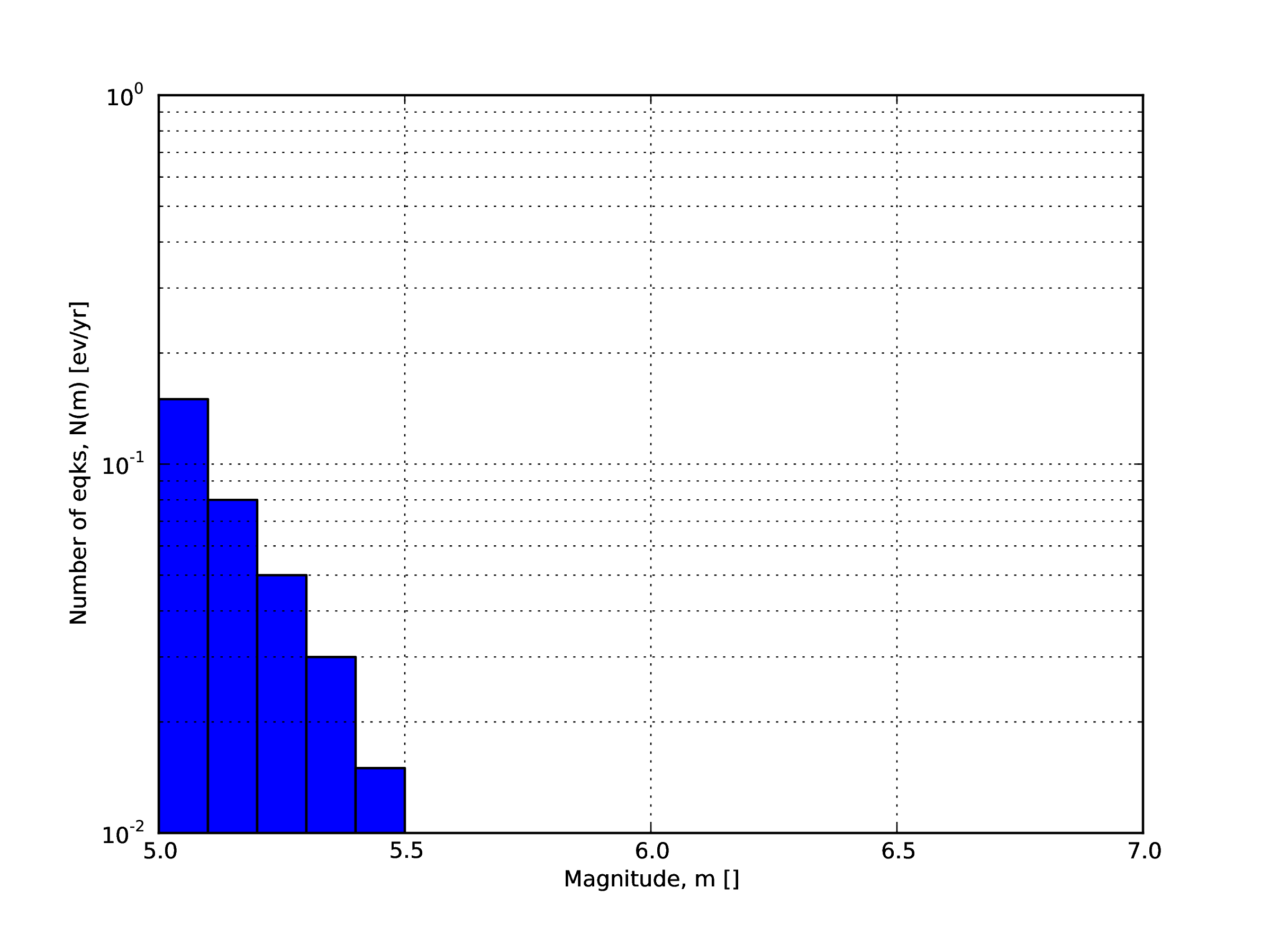
Fig. 2.5 Example of an incremental magnitude-frequency distribution.#
- A double truncated Gutenberg-Richter distribution
This distribution is described by means of a minimum
minMagand maximum magnitudemaxMagand by the \(a\) and \(b\) values of the Gutenberg-Richter relationship.The syntax of the xml used to describe this magnitude-frequency distribution is rather compact as demonstrated in the following example:
1<truncGutenbergRichterMFD aValue="5.0" bValue="1.0" minMag="5.0"
2                          maxMag="6.0"/>
Fig. 2.6 shows the magnitude-frequency distribution obtained using the parameters of the considered example.
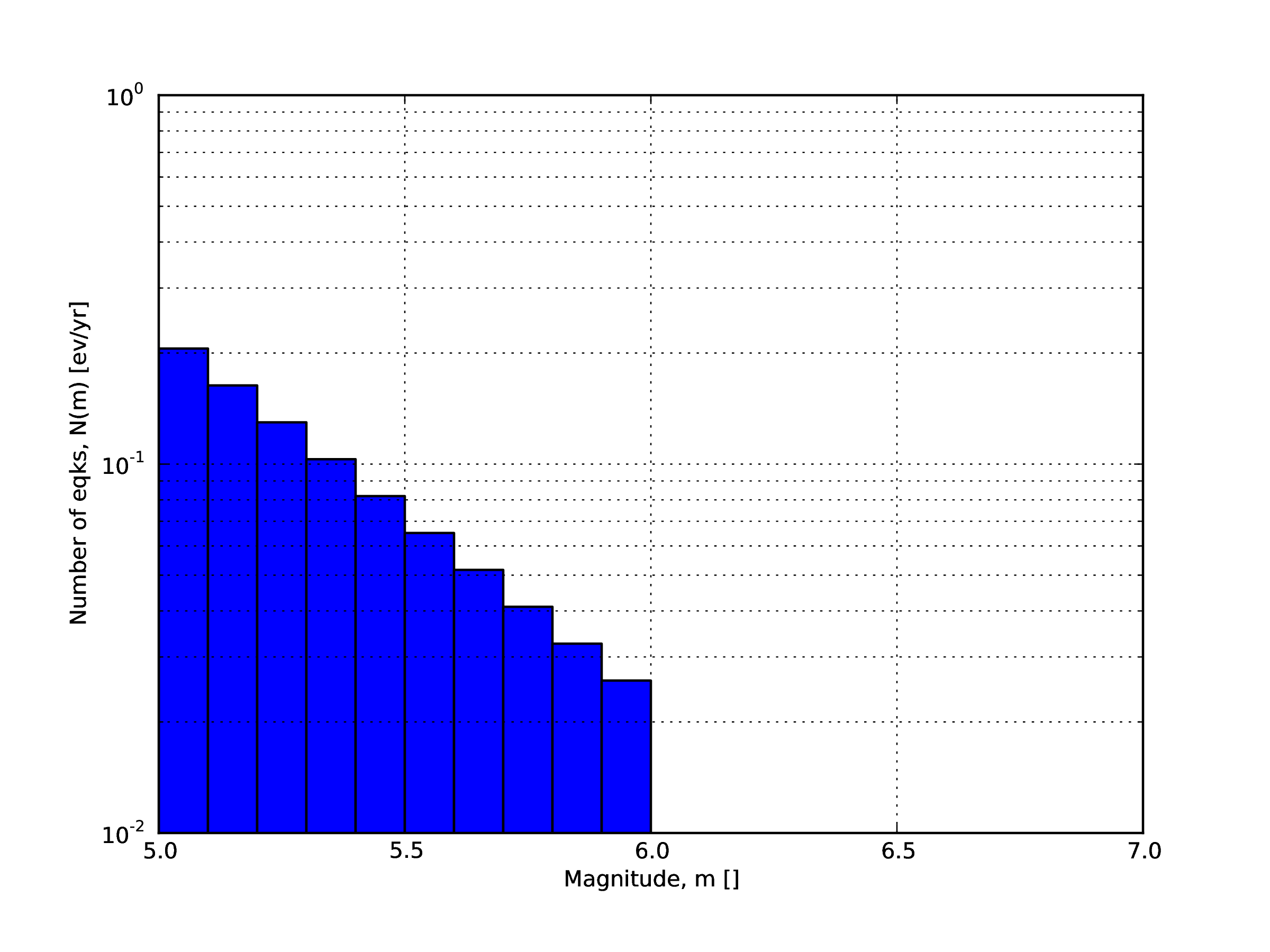
Fig. 2.6 Example of a double truncated Gutenberg-Richter magnitude-frequency distribution.#
- Hybrid Characteristic earthquake model (à la (Youngs and Coppersmith 1985))
The hybrid characteristic earthquake model, presented by (Youngs and Coppersmith 1985), distributes seismic moment proportionally between a characteristic model (for larger magnitudes) and an exponential model. The rate of events is dependent on the magnitude of the characteristic earthquake, the b-value and the total moment rate of the system (Fig. 2.7). However, the total moment rate may be defined in one of two ways. If the total moment rate of the source is known, as may be the case for a fault surface with known area and slip rate, then the distribution can be defined from the total moment rate (in N-m) of the source directly. Alternatively, the distribution can be defined from the rate of earthquakes in the characteristic bin, which may be preferable if the distribution is determined from observed seismicity behaviour. The option to define the distribution according to the total moment rate is input as:
1<YoungsCoppersmithMFD minmag="5.0" bValue="1.0" binWidth="0.1"
2                      characteristicMag="7.0" totalMomentRate="1.05E19"/>
whereas the option to define the distribution from the rate of the characteristic events is given as:
1<YoungsCoppersmithMFD minmag="5.0" bValue="1.0" binWidth="0.1"
2                      characteristicMag="7.0" characteristicRate="0.005"/>
Note that in this distribution the width of the magnitude bin must be defined explicitly in the model.
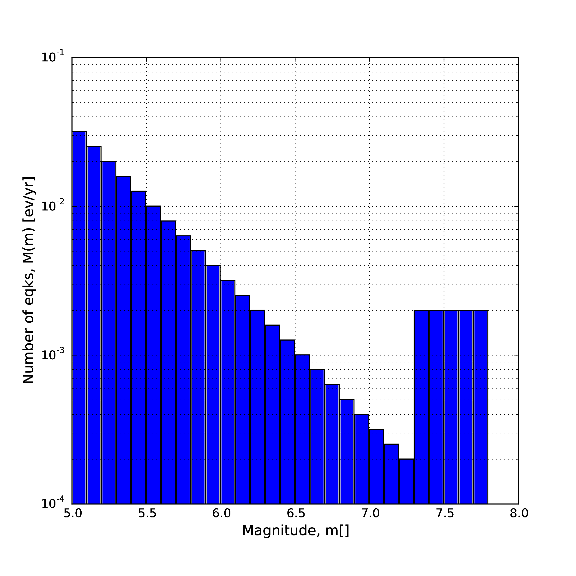
Fig. 2.7 (Youngs and Coppersmith 1985) magnitude-frequency distribution.#
- “Arbitrary” Magnitude Frequency Distribution
The arbitrary magnitude frequency distribution is another non-parametric form of MFD, in which the rates are defined explicitly. Here, the magnitude frequency distribution is defined by a list of magnitudes and their corresponding rates of occurrence. There is no bin-width as the rates correspond exactly to the specific magnitude. Unlike the evenly discretised MFD, there is no requirement that the magnitudes be equally spaced. This distribution (illustrated in Fig. 2.8) can be input as:
1<arbitraryMFD>
2    <occurRates>0.12 0.036 0.067 0.2</occurRates>
3    <magnitudes>8.1 8.47 8.68 9.02</magnitude>
4</arbitraryMFD>
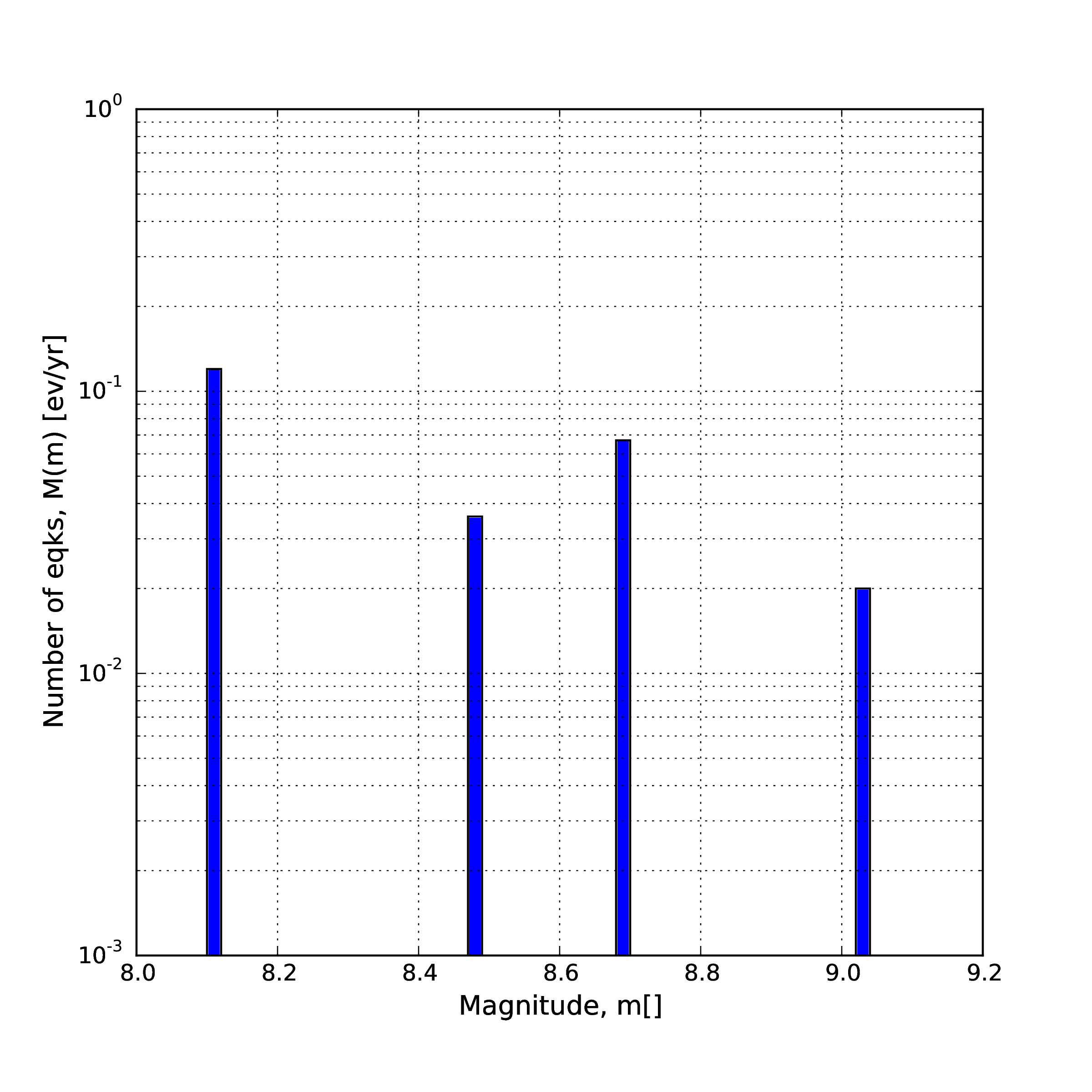
Fig. 2.8 “Arbitrary” magnitude-frequency distribution.#
2.1.3. Magnitude-scaling relationships#
We provide below a list of the magnitude-area scaling relationships implemented in the OpenQuake hazard library (oq-hazardlib):
2.1.3.1. Relationships for shallow earthquakes in active tectonic regions#
(Wells and Coppersmith 1994) - One of the most well known magnitude scaling relationships, based on a global database of historical earthquake ruptures. The implemented relationship is the one linking magnitude to rupture area, and is called with the keyword
WC1994
2.1.3.2. Magnitude-scaling relationships for subduction earthquakes#
(Strasser, Arango, and Bommer 2010) - Defines several magnitude scaling relationships for interface and in-slab earthquakes. Only the magnitude to rupture-area scaling relationships are implemented here, and are called with the keywords
StrasserInterfaceandStrasserIntraslabrespectively.(Thingbaijam, Mai, and Goda 2017) - Define magnitude scaling relationships for interface. Only the magnitude to rupture-area scaling relationships are implemented here, and are called with the keywords
ThingbaijamInterface.
2.1.3.3. Magnitude-scaling relationships stable continental regions#
(EPRI 2011) - Defines a single magnitude to rupture-area scaling relationship for use in the central and eastern United States: \(Area = 10.0^{M_W - 4.336}\). It is called with the keyword
CEUS2011
2.1.3.4. Miscellaneous Magnitude-Scaling Relationships#
PeerMSRdefines a simple magnitude scaling relation used as part of the Pacific Earthquake Engineering Research Center verification of probabilistic seismic hazard analysis programs: \(Area = 10.0 ^{M_W - 4.0}\).PointMSRapproximates a ‘point’ source by returning an infinitesimally small area for all magnitudes. Should only be used for distributed seismicity sources and not for fault sources.
2.1.4. Calculation workflows#
The hazard component of the OpenQuake engine can compute seismic hazard using various approaches. Three types of analysis are currently supported:
Classical Probabilistic Seismic Hazard Analysis (PSHA), allowing calculation of hazard curves and hazard maps following the classical integration procedure ((Cornell 1968), McGuire (1976)) as formulated by (Field, Jordan, and Cornell 2003).
Event-Based Probabilistic Seismic Hazard Analysis, allowing calculation of ground-motion fields from stochastic event sets. Traditional results - such as hazard curves - can be obtained by post- processing the set of computed ground-motion fields.
Scenario Based Seismic Hazard Analysis, allowing the calculation of ground motion fields from a single earthquake rupture scenario taking into account ground-motion aleatory variability.
Each workflow has a modular structure, so that intermediate results can be exported and analyzed. Each calculator can be extended independently of the others so that additional calculation options and methodologies can be easily introduced, without affecting the overall calculation workflow.
2.1.4.1. Classical Probabilistic Seismic Hazard#
Analysis Input data for the classical Probabilistic Seismic Hazard Analysis consist of a PSHA input model provided together with calculation settings.
The main calculators used to perform this analysis are the following:
Logic Tree Processor
The Logic Tree Processor (LTP) takes as an input the Probabilistic Seismic Hazard Analysis Input Model and creates a Seismic Source Model. The LTP uses the information in the Initial Seismic Source Models and the Seismic Source Logic Tree to create a Seismic Source Input Model (i.e. a model describing geometry and activity rates of each source without any epistemic uncertainty).
Following a procedure similar to the one just described the Logic Tree Processor creates a Ground Motion model (i.e. a data structure that associates to each tectonic region considered in the calculation a Ground Motion Prediction Equation).
Earthquake Rupture Forecast Calculator
The produced Seismic Source Input Model becomes an input information for the Earthquake Rupture Forecast (ERF) calculator which creates a list earthquake ruptures admitted by the source model, each one characterized by a probability of occurrence over a specified time span.
Classical PSHA Calculator
The classical PSHA calculator uses the ERF and the Ground Motion model to compute hazard curves on each site specified in the calculation settings.
2.1.4.2. Event-Based Probabilistic Seismic Hazard#
Analysis Input data for the Event-Based PSHA - as in the case of the Classical Probabilistic Seismic Hazard Analysis calculator - consists of a PSHA Input Model and a set of calculation settings.
The main calculators used to perform this analysis are:
Logic Tree Processor
The Logic Tree Processor works in the same way described in the description of the Classical Probabilistic Seismic Hazard Analysis workflow (see Section Classical PSHA).
Earthquake Rupture Forecast Calculator
The Earthquake Rupture Forecast Calculator was already introduced in the description of the PSHA workflow (see Section Classical PSHA).
Stochastic Event Set Calculator
The Stochastic Event Set Calculator generates a collection of stochastic event sets by sampling the ruptures contained in the ERF according to their probability of occurrence.
A Stochastic Event Set (SES) thus represents a potential realisation of the seismicity (i.e. a list of ruptures) produced by the set of seismic sources considered in the analysis over the time span fixed for the calculation of hazard.
Ground Motion Field Calculator
The Ground Motion Field Calculator computes for each event contained in a Stochastic Event Set a realization of the geographic distribution of the shaking by taking into account the aleatory uncertainties in the ground- motion model. Eventually, the Ground Motion Field calculator can consider the spatial correlation of the ground-motion during the generation of the Ground Motion Field.
Event-based PSHA Calculator
The event-based PSHA calculator takes a (large) set of ground-motion fields representative of the possible shaking scenarios that the investigated area can experience over a (long) time span and for each site computes the corresponding hazard curve.
This procedure is computationally intensive and is not recommended for investigating the hazard over large areas.
2.1.4.3. Scenario based Seismic Hazard Analysis#
In case of Scenario Based Seismic Hazard Analysis, the input data consist of a single earthquake rupture model and one or more ground-motion models. Using the Ground Motion Field Calculator, multiple realizations of ground shaking can be computed, each realization sampling the aleatory uncertainties in the ground-motion model. The main calculator used to perform this analysis is the Ground Motion Field Calculator, which was already introduced during the description of the event based PSHA workflow (see Section Event based PSHA).
As the scenario calculator does not need to determine the probability of occurrence of the specific rupture, but only sufficient information to parameterise the location (as a three-dimensional surface), the magnitude and the style-of-faulting of the rupture, a more simplified NRML structure is sufficient compared to the source model structures described previously in Source typologies. A rupture model XML can be defined in the following formats:
Simple Fault Rupture - in which the geometry is defined by the trace of the fault rupture, the dip and the upper and lower seismogenic depths. An example is shown in the listing below:
 1      <?xml version='1.0' encoding='utf-8'?>
 2      <nrml xmlns:gml="http://www.opengis.net/gml"
 3            xmlns="http://openquake.org/xmlns/nrml/0.5">
 4
 5          <simpleFaultRupture>
 6            <magnitude>6.7</magnitude>
 7            <rake>180.0</rake>
 8            <hypocenter lon="-122.02750" lat="37.61744" depth="6.7"/>
 9            <simpleFaultGeometry>
10              <gml:LineString>
11                <gml:posList>
12                  -121.80236 37.39713
13                  -121.91453 37.48312
14                  -122.00413 37.59493
15                  -122.05088 37.63995
16                  -122.09226 37.68095
17                  -122.17796 37.78233
18                </gml:posList>
19              </gml:LineString>
20              <dip>76.0</dip>
21              <upperSeismoDepth>0.0</upperSeismoDepth>
22              <lowerSeismoDepth>13.4</lowerSeismoDepth>
23            </simpleFaultGeometry>
24          </simpleFaultRupture>
25
26      </nrml>
Planar & Multi-Planar Rupture - in which the geometry is defined as a collection of one or more rectangular planes, each defined by four corners. An example of a multi-planar rupture is shown below in the listing below:
 1<?xml version='1.0' encoding='utf-8'?>
 2<nrml xmlns:gml="http://www.opengis.net/gml"
 3      xmlns="http://openquake.org/xmlns/nrml/0.5">
 4
 5    <multiPlanesRupture>
 6        <magnitude>8.0</magnitude>
 7        <rake>90.0</rake>
 8        <hypocenter lat="-1.4" lon="1.1" depth="10.0"/>
 9            <planarSurface strike="90.0" dip="45.0">
10                <topLeft lon="-0.8" lat="-2.3" depth="0.0" />
11                <topRight lon="-0.4" lat="-2.3" depth="0.0" />
12                <bottomLeft lon="-0.8" lat="-2.3890" depth="10.0" />
13                <bottomRight lon="-0.4" lat="-2.3890" depth="10.0" />
14            </planarSurface>
15            <planarSurface strike="30.94744" dip="30.0">
16                <topLeft lon="-0.42" lat="-2.3" depth="0.0" />
17                <topRight lon="-0.29967" lat="-2.09945" depth="0.0" />
18                <bottomLeft lon="-0.28629" lat="-2.38009" depth="10.0" />
19                <bottomRight lon="-0.16598" lat="-2.17955" depth="10.0" />
20            </planarSurface>
21    </multiPlanesRupture>
22
23</nrml>
Complex Fault Rupture - in which the geometry is defined by the upper, lower and (if applicable) intermediate edges of the fault rupture. An example of a complex fault rupture is shown below in the listing below:
 1<?xml version='1.0' encoding='utf-8'?>
 2<nrml xmlns:gml="http://www.opengis.net/gml"
 3      xmlns="http://openquake.org/xmlns/nrml/0.5">
 4
 5    <complexFaultRupture>
 6        <magnitude>8.0</magnitude>
 7        <rake>90.0</rake>
 8        <hypocenter lat="-1.4" lon="1.1" depth="10.0"/>
 9        <complexFaultGeometry>
10            <faultTopEdge>
11                <gml:LineString>
12                    <gml:posList>
13                        0.6 -1.5 2.0
14                        1.0 -1.3 5.0
15                        1.5 -1.0 8.0
16                    </gml:posList>
17                </gml:LineString>
18            </faultTopEdge>
19            <intermediateEdge>
20                <gml:LineString>
21                    <gml:posList>
22                        0.65 -1.55 4.0
23                        1.1  -1.4  10.0
24                        1.5  -1.2  20.0
25                    </gml:posList>
26                </gml:LineString>
27            </intermediateEdge>
28            <faultBottomEdge>
29                <gml:LineString>
30                    <gml:posList>
31                        0.65 -1.7 8.0
32                        1.1  -1.6 15.0
33                        1.5  -1.7 35.0
34                    </gml:posList>
35                </gml:LineString>
36            </faultBottomEdge>
37        </complexFaultGeometry>
38    </complexFaultRupture>
39
40</nrml>
2.2. Using the Hazard Module#
This Chapter summarises the structure of the information necessary to define a PSHA input model to be used with the OpenQuake engine.
Input data for probabilistic based seismic hazard analysis (Classical, Event based, Disaggregation, and Uniform Hazard Spectra) are organised into:
A general configuration file.
A file describing the Seismic Source System, that is the set of initial source models and associated epistemic uncertainties needed to model the seismic activity in the region of interest.
A file describing the Ground Motion System, that is the set of ground motion prediction equations, per tectonic region type, needed to model the ground motion shaking in the region of interest.
Fig. 2.9 summarises the structure of a PSHA input model for the OpenQuake engine and the relationships between the different files.
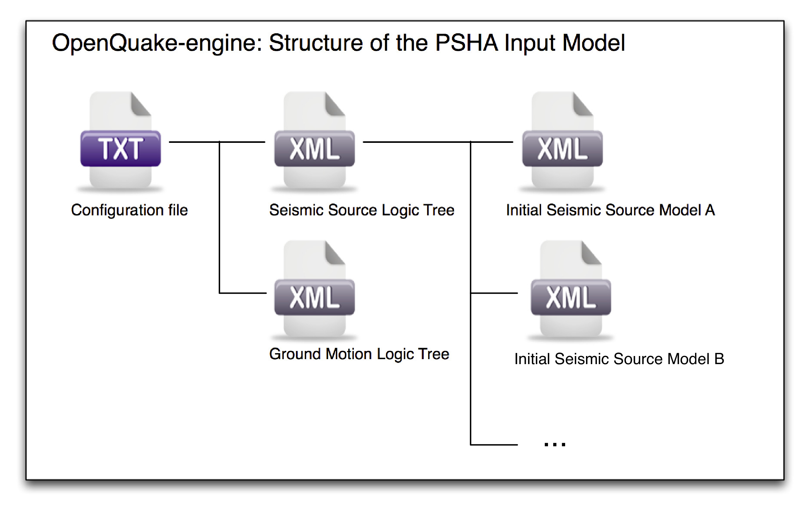
Fig. 2.9 PSHA Input Model structure#
2.2.1. Defining Logic Trees#
The main components of a logic tree structure in the OpenQuake engine are the following:
- Branch
: the simplest component of a logic tree structure. A Branch represent a possible interpretation of a value assignment for a specific type of uncertainty. It is fully described by the tuple (parameter or model, weight).
- Branching set
: it is a key component in the logic tree structure used by the OpenQuake engine. It groups a set of branches i.e. alternative interpretations of a parameter or a model. Each branching set is defined by:
An ID
An uncertainty type (for a comprehensive list of the types of uncertainty currently supported see section Logic trees as described in the nrml schema)
One or more branches
This set of uncertainties can be applied to the whole initial seismic source input model or just to a subset of seismic sources. The sum of the weights/probabilities assigned to the set of branches always correspond to one.
Below we provide a simple schema illustrating the skeleton of xml file containing the desciption of a logic tree:
1    <logicTreeBranchSet branchSetID=ID
2                        uncertaintyType=TYPE>
3        <logicTreeBranch>
4            <uncertaintyModel>VALUE</uncertaintyModel>
5            <uncertaintyWeight>WEIGHT</uncertaintyWeight>
6        </logicTreeBranch>
7    </logicTreeBranchSet>
As it appears from this example, the structure of a logic tree is a set of nested elements.
A schematic representation of the elemental components of a logic tree structure is provided in Fig. 2.10. A Branch set identifies a collection of branches (i.e. individual branches) whose weights sum to 1.
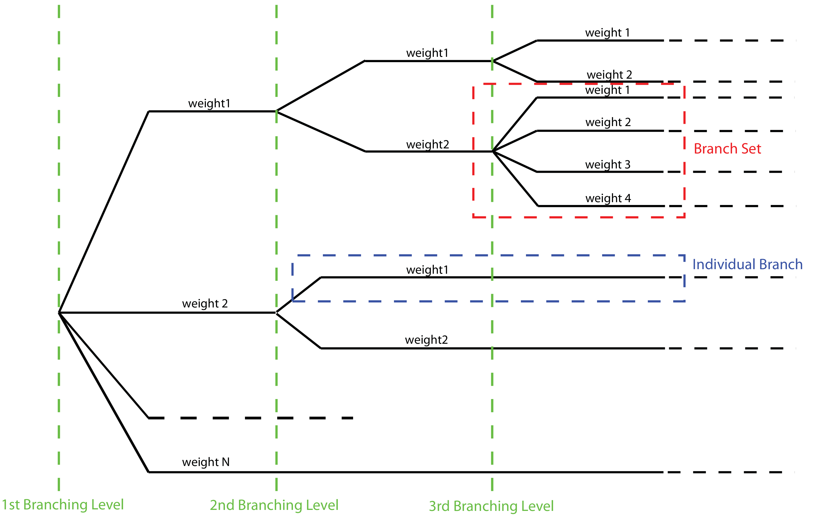
Fig. 2.10 Generic Logic Tree structure as described in terms of Branch sets, and individual branches.#
2.2.1.1. Logic trees as described in the nrml schema#
In the NRML schema, a logic tree structure is defined through the
logicTree element:
1<logicTree logicTreeID="ID">
2...
3</logicTree>
A logicTree contains as a sequence of logicTreeBranchSet
elements.
There are no restrictions on the number of Branch set that can be defined.
Each logicTreeBranchSet has two required attributes: branchSetID
and uncertaintyType. The latter defines the type of epistemic
uncertainty this Branch set is describing.
 1<logicTree logicTreeID="ID">
 2             <logicTreeBranchSet branchSetID="ID_1"
 3                     uncertaintyType="UNCERTAINTY_TYPE">
 4                     ...
 5             </logicTreeBranchSet>
 6             <logicTreeBranchSet branchSetID="ID_2"
 7                     uncertaintyType="UNCERTAINTY_TYPE">
 8                     ...
 9             </logicTreeBranchSet>
10             ...
11             <logicTreeBranchSet branchSetID="ID_N"
12                     uncertaintyType="UNCERTAINTY_TYPE">
13                     ...
14             </logicTreeBranchSet>
15...
16</logicTree>
Possible values for the uncertaintyType attribute are:
gmpeModel: indicates epistemic uncertainties on ground motion prediction equationssourceModel: indicates epistemic uncertainties on source modelsmaxMagGRRelative: indicates relative (i.e. increments) epistemic uncertainties to be added (or subtracted, depending on the sign of the increment) to the Gutenberg-Richter maximum magnitude value.bGRRelative: indicates relative epistemic uncertainties to be applied to the Gutenberg-Richter b value.abGRAbsolute: indicates absolute (i.e. values used to replace original values) epistemic uncertainties on the Gutenberg-Richter a and b values.maxMagGRAbsolute: indicates (absolute) epistemic uncertainties on the Gutenberg-Richter maximum magnitude.incrementalMFDAbsolute: indicates (absolute) epistemic uncertainties on the incremental magnitude frequency distribution (i.e. alternative rates and/or minimum magnitude) of a specific source (can only be applied to individual sources)simpleFaultGeometryAbsolute: indicates alternative representations of the simple fault geometry for an individual simple fault sourcesimpleFaultDipRelative: indicates a relative increase or decrease in fault dip for one or more simple fault sourcessimpleFaultDipAbsolute: indicates alternative values of fault dip for one or more simple fault sourcescomplexFaultGeometryAbsolute: indicates alternative representations of complex fault geometry for an individual complex fault sourcecharacteristicFaultGeometryAbsolute: indicates alternative representations of the characteristic fault geometry for an individual characteristic fault source
A branchSet is defined as a sequence of logicTreeBranch
elements, each specified by an uncertaintyModel element (a string
identifying an uncertainty model; the content of the string varies with
the uncertaintyType attribute value of the branchSet element) and
the uncertaintyWeight element (specifying the probability/weight
associated to the uncertaintyModel):
 1< logicTree  logicTreeID="ID">
 2...
 3
 4             < logicTreeBranchSet  branchSetID="ID_#"
 5                             uncertaintyType="UNCERTAINTY_TYPE">
 6                     < logicTreeBranch  branchID="ID_1">
 7                             <uncertaintyModel>
 8                                 UNCERTAINTY_MODEL
 9                             </uncertaintyModel>
10                             <uncertaintyWeight>
11                                 UNCERTAINTY_WEIGHT
12                             </uncertaintyWeight>
13                     </ logicTreeBranch >
14                     ...
15                     < logicTreeBranch  branchID="ID_N">
16                             <uncertaintyModel>
17                                 UNCERTAINTY_MODEL
18                             </uncertaintyModel>
19                             <uncertaintyWeight>
20                                 UNCERTAINTY_WEIGHT
21                             </uncertaintyWeight>
22                     </logicTreeBranch>
23             </logicTreeBranchSet>
24...
25</logicTree >
Depending on the uncertaintyType the content of the
<uncertaintyModel> element changes:
if
uncertaintyType="gmpeModel", the uncertainty model contains the name of a ground motion prediction equation (a list of available GMPEs can be obtained usingoq info gsimsand these are also documented at: http://docs.openquake.org/oq-engine/stable/openquake.hazardlib.gsim.html):<uncertaintyModel>GMPE_NAME</uncertaintyModel>
if
uncertaintyType="sourceModel", the uncertainty model contains the paths to a source model file, e.g.:1<uncertaintyModel>SOURCE_MODEL_FILE_PATH</uncertaintyModel>
if
uncertaintyType="maxMagGRRelative", the uncertainty model contains the increment to be added (or subtracted, depending on the sign) to the Gutenberg-Richter maximum magnitude:<uncertaintyModel>MAX_MAGNITUDE_INCREMENT</uncertaintyModel>
if
uncertaintyType="bGRRelative", the uncertainty model contains the increment to be added (or subtracted, depending on the sign) to the Gutenberg-Richter b value:<uncertaintyModel>B_VALUE_INCREMENT</uncertaintyModel>
if
uncertaintyType="abGRAbsolute", the uncertainty model must contain one a and b pair:<uncertaintyModel>A_VALUE B_VALUE</uncertaintyModel>
if
uncertaintyType="maxMagGRAbsolute", the uncertainty model must contain one Gutenberg-Richter maximum magnitude value:<uncertaintyModel>MAX_MAGNITUDE</uncertaintyModel>
if
uncertaintyType="incrementalMFDAbsolute", the uncertainty model must contain an instance of the incremental MFD node:1<uncertaintyModel> 2 <incrementalMFD 3 minMag="MIN MAGNITUDE" 4 binWidth="BIN WIDTH"> 5 <occurRates>RATE_1 RATE_2 ... RATE_N</occurRates> 6 </incrementalMFD> 7</uncertaintyModel>
if
uncertaintyType="simpleFaultGeometryAbsolute"then the uncertainty model must contain a valid instance of thesimpleFaultGeometrynode as described in section Simple Faultsif
uncertaintyType="simpleFaultDipRelative"then the uncertainty model must specify the number of degrees to increase (positive) or decrease (negative) the fault dip. Note that if this increase results in an adjusted fault dip greater than \(90^{\circ}\) or less than \(0^{\circ}\) an error will occur.<uncertaintyModel>DIP_INCREMENT</uncertaintyModel>
if
uncertaintyType="simpleFaultDipAbsolute"then the uncertainty model must specify the dip angle (in degrees)<uncertaintyModel>DIP</uncertaintyModel>
if
uncertaintyType="complexFaultGeometryAbsolute"then the uncertainty model must contain a valid instance of thecomplexFaultGeometrysource node as described in section Complex Faultsif
uncertaintyType="characteristicFaultGeometryAbsolute"then the uncertainty model must contain a valid instance of thecharacteristicFaultGeometrysource node, as described in section Characteristic faults
There are no restrictions on the number of logicTreeBranch elements
that can be defined in a logicTreeBranchSet, as long as the
uncertainty weights sum to 1.0.
The logicTreeBranchSet element offers also a number of optional
attributes allowing for complex tree definitions:
applyToBranches: specifies to whichlogicTreeBranchelements (one or more), in the previous Branch sets, the Branch set is linked to. The linking is established by defining the IDs of the branches to link to:applyToBranches="branchID1 branchID2 .... branchIDN"
The default is the keyword ALL, which means that a Branch set is by default linked to all branches in the previous Branch set. By specifying one or more branches to which the Branch set links to, non- symmetric logic trees can be defined.
applyToSources: specifies to which source in a source model the uncertainty applies to. Sources are specified in terms of their IDs:applyToSources="srcID1 srcID2 .... srcIDN"
applyToTectonicRegionType: specifies to which tectonic region type the uncertainty applies to. Only one tectonic region type can be defined (Active Shallow Crust,Stable Shallow Crust,Subduction Interface,SubductionIntraSlab,Volcanic), e.g.:applyToTectonicRegionType="Active Shallow Crust"
2.2.2. The Seismic Source System#
The Seismic Source System contains the model (or the models) describing position, geometry and activity of seismic sources of engineering importance for a set of sites as well as the possible epistemic uncertainties to be incorporated into the calculation of seismic hazard.
2.2.2.1. The Seismic Source Logic Tree#
The structure of the Seismic Source Logic Tree consists of at least one Branch Set. The example provided below shows the simplest Seismic Source Logic Tree structure that can be defined in a Psha Input Model for OpenQuake engine. It’s a logic tree with just onebranchset with one Branch used to define the initial seismic source model (its weight will be equal to one).
 1<?xml version="1.0" encoding="UTF-8"?>
 2<nrml xmlns:gml="http://www.opengis.net/gml"
 3      xmlns="http://openquake.org/xmlns/nrml/0.5">
 4    <logicTree logicTreeID="lt1">
 5            <logicTreeBranchSet uncertaintyType="sourceModel"
 6                                branchSetID="bs1">
 7                <logicTreeBranch branchID="b1">
 8                    <uncertaintyModel>seismic_source_model.xml
 9                    </uncertaintyModel>
10                    <uncertaintyWeight>1.0</uncertaintyWeight>
11                </logicTreeBranch>
12            </logicTreeBranchSet>
13    </logicTree>
14</nrml>
The optional branching levels will contain rules that modify parameters of the sources in the initial seismic source model.
For example, if the epistemic uncertainties to be considered are source geometry and maximum magnitude, the modeller can create a logic tree structure with three initial seismic source models (each one exploring a different definition of the geometry of sources) and one branching level accounting for the epistemic uncertainty on the maximum magnitude.
Below we provide an example of such logic tree structure. Note that the uncertainty on the maximum magnitude is specified in terms of relative increments with respect to the initial maximum magnitude defined for each source in the initial seismic source models.
 1<?xml version="1.0" encoding="UTF-8"?>
 2<nrml xmlns:gml="http://www.opengis.net/gml"
 3      xmlns="http://openquake.org/xmlns/nrml/0.5">
 4    <logicTree logicTreeID="lt1">
 5
 6            <logicTreeBranchSet uncertaintyType="sourceModel"
 7                                branchSetID="bs1">
 8                <logicTreeBranch branchID="b1">
 9                    <uncertaintyModel>seismic_source_model_A.xml
10                    </uncertaintyModel>
11                    <uncertaintyWeight>0.2</uncertaintyWeight>
12                </logicTreeBranch>
13                <logicTreeBranch branchID="b2">
14                    <uncertaintyModel>seismic_source_model_B.xml
15                    </uncertaintyModel>
16                    <uncertaintyWeight>0.3</uncertaintyWeight>
17                </logicTreeBranch>
18                <logicTreeBranch branchID="b3">
19                    <uncertaintyModel>seismic_source_model_C.xml
20                    </uncertaintyModel>
21                    <uncertaintyWeight>0.5</uncertaintyWeight>
22                </logicTreeBranch>
23            </logicTreeBranchSet>
24
25            <logicTreeBranchSet branchSetID="bs21"
26                    uncertaintyType="maxMagGRRelative">
27                <logicTreeBranch branchID="b211">
28                    <uncertaintyModel>+0.0</uncertaintyModel>
29                    <uncertaintyWeight>0.6</uncertaintyWeight>
30                </logicTreeBranch>
31                <logicTreeBranch branchID="b212">
32                    <uncertaintyModel>+0.5</uncertaintyModel>
33                    <uncertaintyWeight>0.4</uncertaintyWeight>
34                </logicTreeBranch>
35            </logicTreeBranchSet>
36
37    </logicTree>
38</nrml>
Starting from OpenQuake engine v2.4, it is also possible to split a source model into several files and read them as if they were a single file. The file names for the different files comprising a source model should be provided in the source model logic tree file. For instance, a source model could be split by tectonic region using the following syntax in the source model logic tree:
 1<?xml version="1.0" encoding="UTF-8"?>
 2<nrml xmlns:gml="http://www.opengis.net/gml"
 3      xmlns="http://openquake.org/xmlns/nrml/0.5">
 4    <logicTree logicTreeID="lt1">
 5            <logicTreeBranchSet uncertaintyType="sourceModel"
 6                                branchSetID="bs1">
 7                <logicTreeBranch branchID="b1">
 8                    <uncertaintyModel>
 9                     active_shallow_sources.xml
10                     stable_shallow_sources.xml
11                    </uncertaintyModel>
12                    <uncertaintyWeight>1.0</uncertaintyWeight>
13                </logicTreeBranch>
14            </logicTreeBranchSet>
15    </logicTree>
16</nrml>
2.2.2.2. The Seismic Source Model#
The structure of the xml file representing the seismic source model corresponds to a list of sources, each one modelled using one out of the five typologies currently supported. Below we provide a schematic example of a seismic source model:
 1<?xml version="1.0" encoding="UTF-8"?>
 2<nrml xmlns:gml="http://www.opengis.net/gml"
 3      xmlns="http://openquake.org/xmlns/nrml/0.5">
 4    <logicTree logicTreeID="lt1">
 5            <logicTreeBranchSet uncertaintyType="sourceModel"
 6                                branchSetID="bs1">
 7                <logicTreeBranch branchID="b1">
 8                    <uncertaintyModel>seismic_source_model.xml
 9                    </uncertaintyModel>
10                    <uncertaintyWeight>1.0</uncertaintyWeight>
11                </logicTreeBranch>
12            </logicTreeBranchSet>
13    </logicTree>
14</nrml>
2.2.3. The Ground Motion System The Ground Motion#
System defines the models and the possible epistemic uncertainties related to ground motion modelling to be incorporated into the calculation.
2.2.3.1. The Ground Motion Logic Tree#
The structure of the Ground-Motion Logic Tree consists of a list of ground motion prediction equations for each tectonic region used to characterise the sources in the PSHA input model.
The example below in shows a simple Ground-Motion Logic Tree. This logic tree assumes that all the sources in the PSHA input model belong to “Active Shallow Crust” and uses for calculation the B. S.-J. Chiou and Youngs (2008) Ground Motion Prediction Equation.
 1<?xml version="1.0" encoding="UTF-8"?>
 2<nrml xmlns:gml="http://www.opengis.net/gml"
 3      xmlns="http://openquake.org/xmlns/nrml/0.5">
 4    <logicTree logicTreeID="lt1">
 5            <logicTreeBranchSet uncertaintyType="gmpeModel"
 6                    branchSetID="bs1"
 7                    applyToTectonicRegionType="Active Shallow Crust">
 8
 9                <logicTreeBranch branchID="b1">
10                    <uncertaintyModel>
11                    ChiouYoungs2008
12                    </uncertaintyModel>
13                    <uncertaintyWeight>1.0</uncertaintyWeight>
14                </logicTreeBranch>
15
16            </logicTreeBranchSet>
17    </logicTree>
18</nrml>
2.2.4. Configuration file#
The configuration file is the primary file controlling both the definition of the input model as well as parameters governing the calculation. We illustrate in the following different examples of the configuration file addressing different types of seismic hazard calculations.
2.2.4.1. Classical PSHA#
In the following we describe the overall structure and the most typical parameters of a configuration file to be used for the computation of a seismic hazard map using a classical PSHA methodology.
Calculation type and model info
1[general]
2description = A demo OpenQuake-engine .ini file for classical PSHA
3calculation_mode = classical
4random_seed = 1024
In this section the user specifies the following parameters:
description: a parameter that can be used to designate the modelcalculation_mode: it is used to set the kind of calculation. In this case it corresponds toclassical. Alternative options for the calculation_mode are described later in this manual.random_seed: is used to control the random generator so that when Monte Carlo procedures are used calculations are replicable (if the samerandom_seedis used you get exactly the same results).
Geometry of the area (or the sites) where hazard is computed
This section is used to specify where the hazard will be computed. Two options are available:
The first option is to define a polygon (usually a rectangle) and a distance (in km) to be used to discretize the polygon area. The polygon is defined by a list of longitude-latitude tuples.
An example is provided below:
5[geometry]
6region = 10.0 43.0, 12.0 43.0, 12.0 46.0, 10.0 46.0
7region_grid_spacing = 10.0
The second option allows the definition of a number of sites where the hazard will be computed. Each site is specified in terms of a longitude, latitude tuple. Optionally, if the user wants to consider the elevation of the sites, a value of depth [km] can also be specified, where positive values indicate below sea level, and negative values indicate above sea level (i.e. the topographic surface). If no value of depth is given for a site, it is assumed to be zero. An example is provided below:
8[geometry]
9sites = 10.0 43.0, 12.0 43.0, 12.0 46.0, 10.0 46.0
If the list of sites is too long the user can specify the name of a csv file as shown below:
10[geometry]
11sites_csv = <name_of_the_csv_file>
The format of the csv file containing the list of sites is a sequence of points (one per row) specified in terms of the longitude, latitude tuple. Depth values are again optional. An example is provided below:
179.0,90.0
178.0,89.0
177.0,88.0
Logic tree sampling
The OpenQuake engine provides two options for processing the whole logic tree structure. The first option uses Montecarlo sampling; the user in this case specifies a number of realizations.
In the second option all the possible realizations are created. Below we
provide an example for the latter option. In this case we set the
number_of_logic_tree_samples to 0. OpenQuake engine will perform a complete
enumeration of all the possible paths from the roots to the leaves of
the logic tree structure.
12[logic_tree]
13number_of_logic_tree_samples = 0
If the seismic source logic tree and the ground motion logic tree do not contain epistemic uncertainties the engine will create a single PSHA input.
Generation of the earthquake rupture forecast
14[erf]
15rupture_mesh_spacing = 5
16width_of_mfd_bin = 0.1
17area_source_discretization = 10
This section of the configuration file is used to specify the level of discretization of the mesh representing faults, the grid used to delineate the area sources and, the magnitude-frequency distribution. Note that the smaller is the mesh spacing (or the bin width) the larger are (1) the precision in the calculation and (2) the computation demand.
In cases where the source model may contain a mixture of simple and complex ruptures it is possible to define a different rupture mesh spacing for complex faults only. This may be helpful in models that permit floating ruptures over large subduction sources, in which the nearest source to site distances may be larger than 20 - 30 km, and for which a small mesh spacing would produce a very large number of ruptures. The spacing for complex faults only can be configured by the line:
18complex_fault_mesh_spacing = 10
Parameters describing site conditions
18[site_params]
19reference_vs30_type = measured
20reference_vs30_value = 760.0
21reference_depth_to_2pt5km_per_sec = 5.0
22reference_depth_to_1pt0km_per_sec = 100.0
In this section the user specifies local soil conditions. The simplest solution is to define uniform site conditions (i.e. all the sites have the same characteristics).
Alternatively it is possible to define spatially variable soil properties in a separate file; the engine will then assign to each investigation location the values of the closest point used to specify site conditions.
23[site_params]
24site_model_file = site_model.csv
The file containing the site model has the following structure:
lon,lat,vs30,z1pt0,z2pt5,vs30measured,backarc
10.0,40.0,800.0,19.367196734,0.588625072259,0,0
10.1,40.0,800.0,19.367196734,0.588625072259,0,0
10.2,40.0,800.0,19.367196734,0.588625072259,0,0
10.3,40.0,800.0,19.367196734,0.588625072259,0,0
10.4,40.0,800.0,19.367196734,0.588625072259,0,0
Notice that the \(0\) for the field vs30measured means that the
vs30 field is inferred, not measured. Most of the GMPEs are not
sensitive to it, so you can usually skip it. For the backarc
parameter \(0\) means false and this is the default, so you can skip
such column. All columns that have defaults or are not needed by the
GMPEs you are using can be skipped, while you will get an error if a
relevant column is missing.
If the closest available site with soil conditions is at a distance greater than 5 km from the investigation location, a warning is generated.
Note: For backward-compatibility reasons, the site model file can also be given in XML format. That old format is deprecated but there are no plans to remove it any soon.
Calculation configuration
25[calculation]
26source_model_logic_tree_file = source_model_logic_tree.xml
27gsim_logic_tree_file = gmpe_logic_tree.xml
28investigation_time = 50.0
29intensity_measure_types_and_levels = {"PGA": [0.005, ..., 2.13]}
30truncation_level = 3
31maximum_distance = 200.0
This section of the OpenQuake engine configuration file specifies the parameters that are relevant for the calculation of hazard. These include the names of the two files containing the Seismic Source System and the Ground Motion System, the duration of the time window used to compute the hazard, the ground motion intensity measure types and levels for which the probability of exceedence will be computed, the level of truncation of the Gaussian distribution of the logarithm of ground motion used in the calculation of hazard and the maximum integration distance (i.e. the distance within which sources will contribute to the computation of the hazard).
The maximum distance refers to the largest distance between a rupture and the target calculation sites in order for the rupture to be considered in the PSHA calculation. This can be input directly in terms of kilometres (as above). There may be cases, however, in which it may be appropriate to have a different maximum source to site distance depending on the tectonic region type. This may be used, for example, to eliminate the impact of small, very far-field sources in regions of high attenuation (in which case maximum distance is reduced), or conversely it may be raised to allow certain source types to contribute to the hazard at greater distances (such as in the case when the region has lower attenuation). An example configuration for a maximum distance in Active Shallow Crust of 150 km, and in Stable Continental Crust of 200 km, is shown below:
31maximum_distance = {'Active Shallow Crust': 150.0,
32                    'Stable Continental Crust': 200.0}
Output
31[output]
32export_dir = outputs/
33# given the specified `intensity_measure_types_and_levels`
34mean = true
35quantiles = 0.1 0.5 0.9
36uniform_hazard_spectra = false
37poes = 0.1
The final section of the configuration file is the one that contains the
parameters controlling the types of output to be produced. Providing an
export directory will tell OpenQuake where to place the output files
when the --exports flag is used when running the program. Setting
mean to true will result in a specific output containing the mean
curves of the logic tree, likewise quantiles will produce separate
files containing the quantile hazard curves at the quantiles listed
(0.1, 0.5 and 0.9 in the example above, leave blank or omit if no
quantiles are required). Setting uniform_hazard_spectra to true will
output the uniform hazard spectra at the same probabilities of
exceedence (poes) as those specified by the later option poes. The
probabilities specified here correspond to the set investigation time.
Specifying poes will output hazard maps. For more information about the
outputs of the calculation, see the section: “Description of hazard
output” (page ).
2.2.4.2. Seismic hazard disaggregation#
In this section we describe the structure of the configuration file to be used to complete a seismic hazard disaggregation. Since only a few parts of the standard configuration file need to be changed we can use the description given in Section Classical PSHA as a reference and we emphasize herein major differences.
1[general]
2description = A demo .ini file for PSHA disaggregation
3calculation_mode = disaggregation
4random_seed = 1024
The calculation mode parameter in this case is set as
disaggregation.
Geometry of the area (or the sites) where hazard is computed
5[geometry]
6sites = 11.0 44.5
In the section it is necessary to specify the geographic coordinates of the site(s) where the disaggregation will be performed. The coordinates of multiple site should be separated with a comma.
Disaggregation parameters
The disaggregation parameters need to be added to the the standard configuration file. They are shown in the following example and a description of each parameter is provided below.
 7[disaggregation]
 8poes_disagg = 0.02, 0.1
 9mag_bin_width = 1.0
10distance_bin_width = 25.0
11coordinate_bin_width = 1.5
12num_epsilon_bins = 3
13disagg_outputs = Mag_Dist_Eps Mag_Lon_Lat
14num_rlzs_disagg = 3
poes_disagg: disaggregation is performed for the intensity measure levels corresponding to the probability of exceedance value(s) provided here. The computations use theinvestigation_timeand theintensity_measure_types_and_levelsdefined in the “Calculation configuration” section (see page ). For thepoes_disaggthe intensity measure level(s) for the disaggregation are inferred by performing a classical calculation and by inverting the hazard curves.iml_disagg: the intensity measure level(s) to be disaggregated can be directly defined by specifyingiml_disagg. Note that a disaggregation computation requires eitherpoes_disaggoriml_disaggto be defined, but both cannot be defined at the same time.mag_bin_width: mandatory; specifies the width of every magnitude histogram bin of the disaggregation matrix computeddistance_bin_width: specifies the width of every distance histogram bin of the disaggregation matrix computed (km)coordinate_bin_width: specifies the width of every longitude-latitude histogram bin of the disaggregation matrix computed (decimal degrees)num_epsilon_bins: mandatory; specifies the number of Epsilon histogram bins of the disaggregation matrix. The width of the Epsilon bins depends on thetruncation_leveldefined in the “Calculation configuration” section (page )disagg_outputs: optional; specifies the type(s) of disaggregation to be computed. The options are:Mag,Dist,Lon_Lat,Lon_Lat_TRT,Mag_Dist,Mag_Dist_Eps,Mag_Lon_Lat,TRT. If none are specified, then all are computed. More details of the disaggregation output are given in the “Outputs from Hazard Disaggregation” section, see page )disagg_by_src: optional; if specified and set to true, disaggregation by source is computed, if possible.num_rlzs_disagg: optional; specifies the number of realizations to be used, selecting those that yield intensity measure levels closest to the mean.
Alternatively to num_rlzs_disagg, the user can specify the index or
indices of the realizations to disaggregate as a list of comma-separated
integers. For example:
7[disaggregation]
8rlz_index = 22,23
If num_rlzs_disagg is specified, the user cannot specify
rlz_index, and vice versa. If num_rlzs_disagg or rlz_index
are specified, the mean disaggregation is automatically computed from
the selected realizations. If neither is specified, the realization that
yields the intensity measure level closest to the mean level will be
selected.
As mentioned above, the user also has the option to perform disaggregation by directly specifying the intensity measure level to be disaggregated, rather than specifying the probability of exceedance. An example is shown below:
7[disaggregation]
8iml_disagg = {'PGA': 0.1}
If iml_disagg is specified, the user should not include
intensity_measure_types_and_levels in the “Calculation
configuration” section (see page ) since it is explicitly given here.
The OQ Engine supports the calculation of two typologies of disaggregation result involving \(\epsilon\). The standard approach used by the OQ Engine is described in the OQ Engine Underlying Hazard Science Book . The reader interested in learning more about the \(\epsilon^*\) can refer to the PEER report Probabilistic Seismic Hazard Analysis Code Verification, PEER Report 2018-03 .
To obtain disaggregation results in terms of \(\epsilon\)* the additional line below must be added to the disaggregation section of the configuration file:
7[disaggregation]
8epsilon_star = True
2.2.4.3. Event based PSHA#
In the following we describe the sections of the configuration file that are required to complete event based PSHA calculations
Calculation type and model info
This part is almost identical to the corresponding one described in Section Classical PSHA.
Note the setting of the calculation_mode parameter which now
corresponds to event_based.
1[general]
2description = A demo OpenQuake-engine .ini file for event based PSHA
3calculation_mode = event_based
4random_seed = 1024
Event based parameters
This section is used to specify the number of stochastic event sets to
be generated for each logic tree realisation (each stochastic event set
represents a potential realisation of seismicity during the
investigation_time specified in the calculation_configuration
part). Additionally, in this section the user can specify the spatial
correlation model to be used for the generation of ground motion fields.
ses_per_logic_tree_path = 5
ground_motion_correlation_model = JB2009
ground_motion_correlation_params = {"vs30_clustering": True}
The acceptable flags for the parameter vs30_clustering are False
and True, with a capital F and T respectively. 0 and
1 are also acceptable flags.
Output
This part substitutes the Output part described in the configuration
file example described in the Section Classical PSHA.
[output]
export_dir = /tmp/xxx
ground_motion_fields = true
# post-process ground motion fields into hazard curves,
# given the specified `intensity_measure_types_and_levels`
hazard_curves_from_gmfs = true
mean = true
quantiles = 0.15, 0.50, 0.85
poes = 0.1, 0.2
Starting from OpenQuake engine22, it is now possible to export information about the ruptures directly in CSV format.
The option hazard_curves_from_gmfs instructs the user to use the
event- based ground motion values to provide hazard curves indicating
the probabilities of exceeding the intensity measure levels set
previously in the intensity_measure_types_and_levels option.
2.2.4.4. Scenario hazard#
In order to run this
calculator, the parameter calculation_mode needs to be set to
scenario. The basic job configuration file required for running a
scenario hazard calculation is shown in
the listing below.
[general]
description = Scenario Hazard Config File
calculation_mode = scenario

[sites]
sites_csv = sites.csv

[rupture]
rupture_model_file = rupture_model.xml
rupture_mesh_spacing = 2.0

[site_params]
site_model_file = site_model.xml

[correlation]
ground_motion_correlation_model = JB2009
ground_motion_correlation_params = {"vs30_clustering": True}

[hazard_calculation]
intensity_measure_types = PGA, SA(0.3), SA(1.0)
random_seed = 42
truncation_level = 3.0
maximum_distance = 200.0
gsim = BooreAtkinson2008
number_of_ground_motion_fields = 1000
Most of the job configuration parameters required for running a scenario
hazard calculation seen in the example in
the listing <lst:config_scenario_hazard> above
are the same as those described in the previous sections for the
classical PSHA calculator
(Section Classical PSHA)
and the event-based PSHA calculator
(Section Event based PSHA).
The set of sites at which the ground motion fields will be produced can
be specifed by using either the sites or sites_csv parameters,
or the region and region_grid_spacing parameters, similar to the
classical PSHA and event-based PSHA calculators. The parameter unique to
the scenario calculator is described below:
number_of_ground_motion_fields: this parameter is used to specify the number of Monte Carlo simulations of the ground motion values at the specified sitesgsim: this parameter indicates the name of a ground motion prediction equation (a list of available GMPEs can be obtained usingoq info gsimsand these are also documented at: http://docs.openquake.org/oq-engine/stable/openquake.hazardlib.gsim.html)
Multiple ground motion prediction equations can be used for a scenario
hazard calculation by providing a GMPE logic tree file (described
previously in Section The Ground Motion Logic Tree) using the
parameter gsim_logic_tree_file. In this case, the OpenQuake engine generates
ground motion fields for all GMPEs specified in the logic tree file. The
Branch weights in the logic tree file are ignored in a scenario analysis
and only the individual Branch results are computed. Mean or quantile
ground motion fields will not be generated.
The ground motion fields will be computed at each of the sites and for each of the intensity measure types specified in the job configuration file. The above calculation can be run using the command line:
user@ubuntu:~$ oq engine --run job.ini
After the calculation is completed, a message similar to the following will be displayed:
Calculation 260 completed in 3 seconds. Results:
  id | name
 569 | Ground Motion Fields
2.3. Hazard Calculations and Results#
In this Chapter we provide a desciption of the main commands available for running hazard with the OpenQuake engine and the file formats used to represent the results of the analyses.
A general introduction on the use of the OpenQuake engine is provided in OpenQuake-engine Background. The reader is invited to consult this part before diving into the following sections.
2.3.1. Running OpenQuake-engine for hazard calculations#
The execution of a hazard analysis using the OpenQuake-engine is
straightforward. Below we provide an example of the simplest command
that can be used to launch a hazard calculation. It consists in the
invocation of oq engine together with the --run option, and the
name of a configuration file (in the example below it corresponds to
job.ini):
user@ubuntu:$ oq engine --run job.ini
The amount of information prompted during the execution of the analysis
can be controlled through the --log-level flag as shown in the
example below:
user@ubuntu:$ oq engine --run job.ini --log-level debug
In this example we ask the engine to provide an extensive amount of
information (usually not justified for a standard analysis). Alternative
options are: debug, info, warn, error, critical.
2.3.2. Exporting results from a hazard calculation#
There are two alternative ways to get results from the OpenQuake-engine: directly through the calculation or by exporting them from the internal OpenQuake engine database once a calculation is completed.
The first option is defined at the OpenQuake-engine invocation through
the flag –exports xml, as shown in the example below:
user@ubuntu:~$ oq engine --run job.ini --exports xml
This will export the results to the results directory specified in
the job.ini file.
The second option allows the user to export the computed results or just
a subset of them whenever they want. In order to obtain the list of
results of the hazard calculations stored in the OpenQuake engine database the
user can utilize the --lhc command (‘list hazard calculations’) to
list the hazard calculations:
user@ubuntu:~$ oq engine --lhc
The execution of this command will produce a list similar to the one provided below (the numbers in red are the calculations IDs):
user@ubuntu:~$ oq engine --lhc
job_id | status | start_time | description
1 | failed | 2013-03-01 09:49:34 | Classical PSHA
2 | successful | 2013-03-01 09:49:56 | Classical PSHA
3 | failed | 2013-03-01 10:24:04 | Classical PSHA
4 | failed | 2013-03-01 10:28:16 | Classical PSHA
5 | failed | 2013-03-01 10:30:04 | Classical PSHA
6 | successful | 2013-03-01 10:31:53 | Classical PSHA
7 | failed | 2013-03-09 08:15:14 | Classical PSHA
8 | successful | 2013-03-09 08:18:04 | Classical PSHA
Subsequently the user can get the list of result stored for a specific
hazard analysis by using the --list-outputs, or --lo, command,
as in the example below (note that the number in blue emphasizes the
result ID):
user@ubuntu:~$ oq engine --lo <calc_id>
id | name
3 | hcurves
and finally extract an xml file for a specific hazard result:
user@ubuntu:~$ oq engine --export-outputs <result_id> <output_folder>
2.3.3. Description of hazard outputs#
The results generated by the OpenQuake-engine are fundamentally of two distinct typologies differentiated by the presence (or absence) of epistemic uncertainty in the PSHA input model.
When epistemic uncertainty is incorporated into the calculation, the OpenQuake-engine calculators (e.g. Classical PSHA, Event Based PSHA, Disaggregation, UHS) produce a set of results (i.e. hazard curves, ground motion fields, disaggregation outputs, UHS, for each logic-tree realisation) which reflects epistemic uncertainties introduced in the PSHA input model. For each logic tree sample, results are computed and stored. Calculation of results statistics (mean, standard deviation, quantiles) are supported by all the calculators.
By default, OpenQuake will export only the statistical results, i.e. mean curves and quantiles. If the user requires the complete results for all realizations, there is a flag to specify, please see the FAQ gem/oq-engine. Beware that if the logic tree contains a large number of end branches the process of exporting the results from each end Branch can add a significant amount of time - possibly longer than the computation time - and result in a large volume of disk spaced being used. In this case it is best to postprocess the data programmatically. Please contact us and we will be happy to give directions on how to do that in Python.
NB: in the literature there are different algorithms for the computation of the quantiles. The OpenQuake engine uses an algorithm based on interpolation which is implemented here:
In particular, the median is computed as the q=0.5 quantile.
2.3.3.1. Outputs from Classical PSHA#
By default, the classical PSHA calculator computes and stores hazard curves for each logic tree sample considered.
When the PSHA input model doesn’t contain epistemic uncertainties the
results is a set of hazard curves (one for each investigated site). The
command below illustrates how is possible to retrieve the group of
hazard curves obtained for a calculation with a given identifier
<calc_id> (see
Section Exporting results from a hazard calculation
for an explanation about how to obtain the list of calculations
performed with their corresponding ID):
user@ubuntu:~$ oq engine --lo <calc_id>
id | name
*3 | Hazard Curves
4 | Realizations
To export from the database the outputs (in this case hazard curves) contained in one of the output identifies, one can do so with the following command:
user@ubuntu:~$ oq engine --export-output <output_id> <output_directory>
Alternatively, if the user wishes to export all of the outputs
associated with a particular calculation then they can use the
--export-outputs with the corresponding calculation key:
user@ubuntu:~$ oq engine --export-outputs <calc_id> <output_directory>
The exports will produce one or more nrml files containing the seismic hazard curves, as represented below in the listing <lst:output_hazard_curves_xml> below.
 1<?xml version="1.0" encoding="utf-8"?>
 2<nrml xmlns:gml="http://www.opengis.net/gml"
 3      xmlns="http://openquake.org/xmlns/nrml/0.5">
 4  <hazardCurves sourceModelTreePath="b1|b212"
 5                gsimTreePath="b2" IMT="PGA"
 6                investigationTime="50.0">
 7    <IMLs>0.005 0.007 0.0098 ... 1.09 1.52 2.13</IMLs>
 8    <hazardCurve>
 9      <gml:Point>
10        <gml:pos>10.0 45.0</gml:pos>
11      </gml:Point>
12      <poEs>1.0 1.0 1.0 ... 0.000688359310522 0.0 0.0</poEs>
13    </hazardCurve>
14    ...
15    <hazardCurve>
16      <gml:Point>
17        <gml:pos>lon lat</gml:pos>
18      </gml:Point>
19      <poEs>poe1 poe2 ... poeN</poEs>
20    </hazardCurve>
21  </hazardCurves>
22</nrml>
Notwithstanding the intuitiveness of this file, let’s have a brief overview of the information included. The overall content of this file is a list of hazard curves, one for each investigated site, computed using a PSHA input model representing one possible realisation obtained using the complete logic tree structure.
The attributes of the hazardCurves element (see text in red) specify
the path of the logic tree used to create the seismic source model
(sourceModelTreePath) and the ground motion model (gsimTreePath)
plus the intensity measure type and the investigation time used to
compute the probability of exceedance.
The IMLs element (in green in the example) contains the values of
shaking used by the engine to compute the probability of exceedance in
the investigation time. For each site this file contains a
hazardCurve element which has the coordinates (longitude and
latitude in decimal degrees) of the site and the values of the
probability of exceedance for all the intensity measure levels specified
in the IMLs element.
If the hazard calculation is configured to produce results including seismic hazard maps and uniform hazard spectra, then the list of outputs would display the following:
user@ubuntu:~$ oq engine --lo <calc_id>
id | name
2 | Full Report
3 | Hazard Curves
4 | Hazard Maps
5 | Realizations
6 | Uniform Hazard Spectra
The first listing below shows a sample of the nrml file used to describe a hazard map, and and the second listing below shows a sample of the nrml used to describe a uniform hazard spectrum.
 1<?xml version="1.0" encoding="UTF-8"?>
 2<nrml xmlns:gml="http://www.opengis.net/gml"
 3      xmlns="http://openquake.org/xmlns/nrml/0.5">
 4  <hazardMap sourceModelTreePath="b1" gsimTreePath="b1"
 5             IMT="PGA" investigationTime="50.0" poE="0.1">
 6    <node lon="119.596690957" lat="21.5497682591" iml="0.204569990197"/>
 7    <node lon="119.596751048" lat="21.6397004197" iml="0.212391638188"/>
 8    <node lon="119.596811453" lat="21.7296325803" iml="0.221407505615"/>
 9    ...
10  </hazardMap>
11</nrml>
 1<?xml version="1.0" encoding="UTF-8"?>
 2<nrml xmlns:gml="http://www.opengis.net/gml"
 3      xmlns="http://openquake.org/xmlns/nrml/0.5">
 4    <uniformHazardSpectra sourceModelTreePath="b1_b2_b4"
 5                        gsimTreePath="b1_b2"
 6                        investigationTime="50.0" poE="0.1">
 7        <periods>0.0 0.025 0.1 0.2</periods>
 8        <uhs>
 9            <gml:Point>
10                <gml:pos>0.0 0.0</gml:pos>
11            </gml:Point>
12            <IMLs>0.3 0.5 0.2 0.1</IMLs>
13        </uhs>
14        <uhs>
15            <gml:Point>
16                <gml:pos>0.0 1.0</gml:pos>
17            </gml:Point>
18            <IMLs>0.3 0.5 0.2 0.1</IMLs>
19        </uhs>
20    </uniformHazardSpectra>
21</nrml>
2.3.3.2. Outputs from Hazard Disaggregation#
The OpenQuake engine output of a disaggregation analysis corresponds to the combination of a hazard curve and a multidimensional matrix containing the results of the disaggregation. For a typical disaggregation calculation the list of outputs are the following:
user@ubuntu:~$ oq engine --lo <calc_id>
id | name
**3** | Disaggregation Outputs
5 | Full Report
6 | Realizations
Running --export-output to export the disaggregation results will
produce individual files for each site. In presence of a nontrivial
logic tree the user can specify the realization on which to perform the
disaggregation by setting the rlz_index parameter in the job.ini
file. If not specified, for each site the engine will determine the
realization closest to the mean hazard curve and will use that
realization to perform the disaggregation.
2.3.3.3. Outputs from Event Based PSHA#
The Event Based PSHA calculator computes and stores stochastic event sets and the corresponding ground motion fields. This calculator can also produce hazard curves and hazard maps, similar to the Classical PSHA calculator. The inset below shows an example of the list of results provided by the OpenQuake engine at the end of an event-based PSHA calculation:
user@ubuntu:~$ oq engine --lo <calc_id>
id | name
10 | Ground Motion Fields
11 | Hazard Curves
12 | Hazard Maps
13 | Realizations
14 | Earthquake Ruptures
15 | Events
16 | Uniform Hazard Spectra
Exporting the outputs from the ruptures will produce a CSV file with the following colums:
rup_id: incremental number identifying the rupturemultiplicity: how many times the rupture occurs in the effective investigation timemag: float specifying the magnitude of the rupturecentroid_lon: longitude of the centroid of the rupturecentroid_lat: latitude of the centroid of the rupturecentroid_depth: depth (in km) of the centroid of the rupturetrt: string specifying the tectonic region typestrike: strike angle of the rupture surfacedip: dip angle of the rupture surfacerake: rake angle of the rupture surface
The outputs from the Ground Motion Fields can be exported in the csv format. Exporting the outputs from the Ground Motion Fields in the csv format results in two csv files illustrated in the example files in Table 2.1 and Table 2.4. The sites csv file provides the association between the site ids in the Ground Motion Fields csv file with their latitude and longitude coordinates.
rlz_id |
site_id |
event_id |
gmv_PGA |
gmv_SA(0.3) |
gmv_SA(1.0) |
|---|---|---|---|---|---|
0 |
0 |
48 |
0.0089 |
0.0686 |
0.0065 |
0 |
0 |
54 |
0.0219 |
0.0325 |
0.0164 |
… |
… |
… |
… |
… |
… |
0 |
6 |
75 |
0.0246 |
0.0244 |
0.0036 |
1 |
0 |
76 |
0.0189 |
0.0327 |
0.0094 |
1 |
0 |
77 |
0.0286 |
0.0683 |
0.0471 |
… |
… |
… |
… |
… |
… |
… |
… |
… |
… |
… |
… |
7 |
6 |
1754 |
0.3182 |
1.2973 |
0.6127 |
7 |
6 |
1755 |
0.2219 |
0.6200 |
0.5069 |
The Events output produces a csv file with fields event_id,
rup_id and rlz_id. The event_id is a 32 bit integer that
identifies uniquely the event; the rup_id is a 32 bit integer that
identifies uniquely the rupture; the rlz_id is a 16 bit integer that
identifies uniquely the realization. The association between the
event_id and the rup_id is stored inside the Events output.
The Realizations output produces a csv file listing the source model
and the combination of ground shaking intensity models for each path
sampled from the logic tree. An example of such a file is shown below in
Table 2.2.
ordinal |
branch_path |
weight |
|---|---|---|
0 |
b1\(\sim\)b11_b21 |
0.1125 |
1 |
b1\(\sim\)b11_b22 |
0.075 |
2 |
b1\(\sim\)b12_b21 |
0.0375 |
3 |
b1\(\sim\)b12_b22 |
0.025 |
4 |
b2\(\sim\)b11_b21 |
0.3375 |
5 |
b2\(\sim\)b11_b22 |
0.225 |
6 |
b2\(\sim\)b12_b21 |
0.1125 |
7 |
b2\(\sim\)b12_b22 |
0.075 |
2.3.3.4. Outputs from Scenario Hazard Analysis#
By default, the scenario hazard calculator computes and stores Ground Motion Fields for each GMPE specified in the job configuration file. The Ground Motion Fields will be computed at each of the sites and for each of the intensity measure types specified in the job configuration file.
Exporting the outputs from the Ground Motion Fields in the csv format results in two csv files illustrated in the example files in Table 2.3 and Table 2.4. The sites csv file provides the association between the site ids in the Ground Motion Fields csv file with their latitude and longitude coordinates.
rlzi |
sid |
eid |
gmv_PGA |
gmv_SA(0.3) |
gmv_SA(1.0) |
|---|---|---|---|---|---|
0 |
0 |
0 |
0.062 |
0.119 |
0.157 |
0 |
1 |
0 |
0.086 |
1.533 |
0.260 |
0 |
2 |
0 |
0.223 |
1.647 |
0.232 |
… |
… |
… |
… |
… |
… |
1 |
4 |
99 |
2.467 |
0.750 |
1.918 |
1 |
5 |
99 |
0.601 |
0.828 |
2.272 |
1 |
6 |
99 |
0.514 |
0.340 |
1.202 |
In this example, the gmfs have been computed using two different GMPEs, so the realization indices (’rlzi’) in the first column of the example gmfs file are either 0 or 1. The gmfs file lists the ground motion values for 100 simulations of the scenario, so the event indices (’eid’) in the third column go from 0–99. There are seven sites with indices 0–6 (’sid’) which are repeated in the second column for each of the 100 simulations of the event and for each of the two GMPEs. Finally, the subsequent columns list the ground motion values for each of the intensity measure types specified in the job configuration file.
site_id |
lon |
lat |
|---|---|---|
0 |
-122.57000 |
38.11300 |
1 |
-122.11400 |
38.11300 |
2 |
-122.00000 |
37.91000 |
3 |
-122.00000 |
38.00000 |
4 |
-122.00000 |
38.11300 |
5 |
-122.00000 |
38.22500 |
6 |
-121.88600 |
38.11300 |
2.4. Demonstrative Examples#
A number of hazard calculation demos are provided with the OpenQuake engine installation,showing different examples of input and configuration files, for different use cases.
This is the list of demos which illustrate how to use the OpenQuake engine for various seismic hazard analysis:
AreaSourceClassicalPSHA
CharacteristicFaultSourceCase1ClassicalPSHA
CharacteristicFaultSourceCase2ClassicalPSHA
CharacteristicFaultSourceCase3ClassicalPSHA
ComplexFaultSourceClassicalPSHA
Disaggregation
EventBasedPSHA
LogicTreeCase1ClassicalPSHA
LogicTreeCase2ClassicalPSHA
LogicTreeCase3ClassicalPSHA
PointSourceClassicalPSHA
SimpleFaultSourceClassicalPSHA
2.4.1. Classical PSHA Demos#
A number of demos have been designed to show how to perform a classical PSHA calculation using the different available source typologies and how to define non-trivial logic trees. It should be noted that the input files that will be illustrated are valid not only for a classical PSHA calculation but also for event based and disaggregation analysis.
All the classical PSHA demos illustrating the different source typologies (all demos but the ones about Logic Tree definition) share the same GSIM logic tree file, which for clarity is provided in the listing below.
Since this logic tree consideres only one tectonic region (i.e.
Active Shallow Crust) all the seismic sources will belong be
considered active shallow crust sources.
 1<?xml version="1.0" encoding="UTF-8"?>
 2<nrml xmlns:gml="http://www.opengis.net/gml"
 3      xmlns="http://openquake.org/xmlns/nrml/0.5">
 4    <logicTree logicTreeID="lt1">
 5            <logicTreeBranchSet uncertaintyType="gmpeModel"
 6                    branchSetID="bs1"
 7                    applyToTectonicRegionType="Active Shallow Crust">
 8
 9                <logicTreeBranch branchID="b1">
10                    <uncertaintyModel>
11                    ChiouYoungs2008
12                    </uncertaintyModel>
13                    <uncertaintyWeight>1.0</uncertaintyWeight>
14                </logicTreeBranch>
15
16            </logicTreeBranchSet>
17    </logicTree>
18</nrml>
2.4.1.1. Classical PSHA with different source typologies#
This section discusses the following examples:
AreaSourceClassicalPSHA
CharacteristicFaultSourceCase1ClassicalPSHA
CharacteristicFaultSourceCase2ClassicalPSHA
CharacteristicFaultSourceCase3ClassicalPSHA
ComplexFaultSourceClassicalPSHA
PointSourceClassicalPSHA
SimpleFaultSourceClassicalPSHA
The configuration file in the listing is defined to compute hazard curves for several intensity measure types (PGV, PGA and Spectral acceleration at different periods), hazard maps and uniform hazard spectra for different probabilities of exceedance:
[general]
description = ...
calculation_mode = classical
random_seed = 23

[geometry]
region = ...
region_grid_spacing = 5.0

[logic_tree]
number_of_logic_tree_samples = 0

[erf]
rupture_mesh_spacing = 2
width_of_mfd_bin = 0.1
area_source_discretization = 5.0

[site_params]
reference_vs30_type = measured
reference_vs30_value = 600.0
reference_depth_to_2pt5km_per_sec = 5.0
reference_depth_to_1pt0km_per_sec = 100.0

[calculation]
source_model_logic_tree_file = source_model_logic_tree.xml
gsim_logic_tree_file = gmpe_logic_tree.xml
investigation_time = 50.0
intensity_measure_types_and_levels = {"PGV": [2, 4, 6 ,8, 10, ...],
                                      "PGA": [0.005, 0.007, ...],
                                      "SA(0.025)": [...],
                                      "SA(0.05)": [...],
                                      "SA(0.1)": [...],
                                      "SA(0.2)": [...],
                                      "SA(0.5)": [...],
                                      "SA(1.0)": [...],
                                      "SA(2.0)": [...]}
truncation_level = 3
maximum_distance = 200.0

[output]
mean = false
quantiles = 0.15, 0.50, 0.85
hazard_maps = true
uniform_hazard_spectra = true
poes = 0.10, 0.02
Hazard maps (for PGA, 10% in 50 years) for the different demos using various oq-engine source typologies are shown in the figures below:

Fig. 2.11 Point Source (a).#
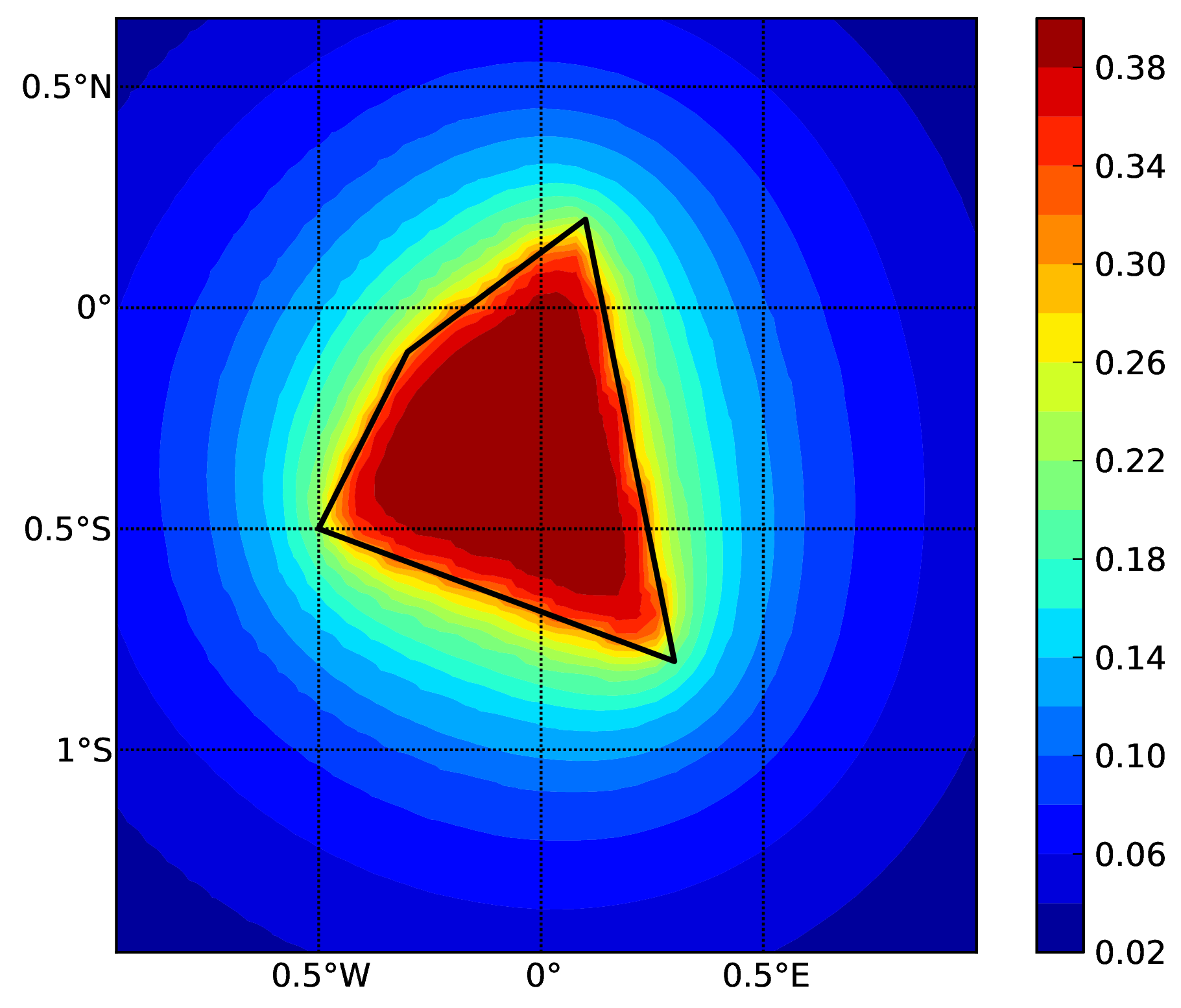
Fig. 2.12 Area source (b). The solid black line represents the area boundary.#
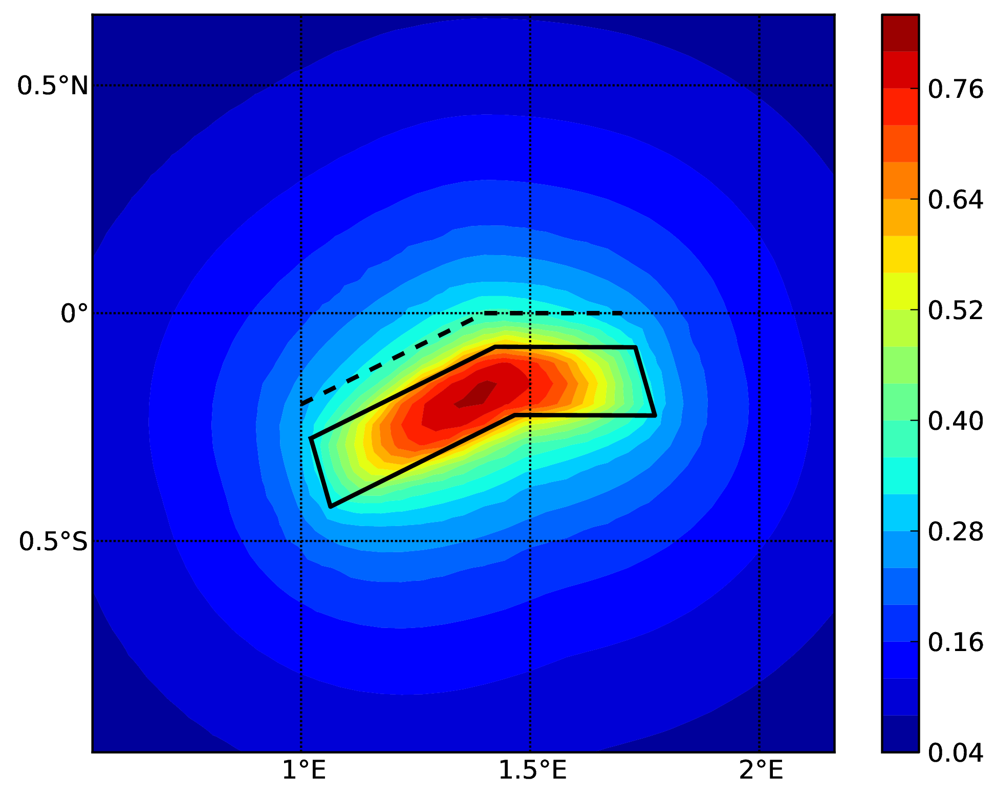
Fig. 2.13 Simple Fault Source (c). The dashed line represents the fault trace, while the solid line the fault surface projection.#
Fig. 2.14 (d) Complex Fault Source. The solid line represent the fault surface projection#
Hazard maps (for PGA, 10% in 50 years) as obtained from characteristic fault sources with simple fault geometry (a), complex fault geometry (b), and collection of planar surfaces (c)
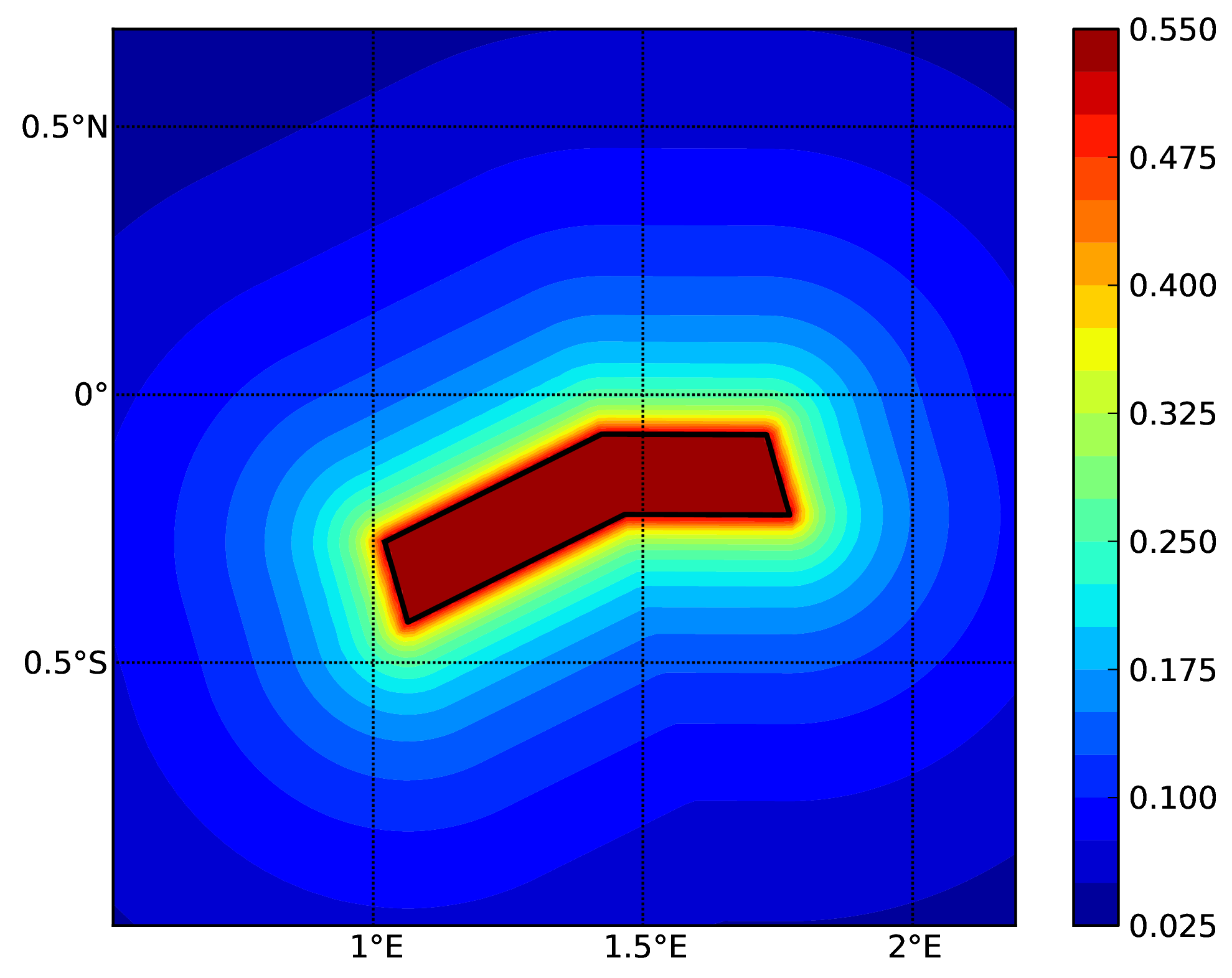
Fig. 2.15 characteristic fault source with simple fault geometry#

Fig. 2.16 characteristic fault source with complex fault geometry#

Fig. 2.17 characteristic fault source with collection of planar surfaces#
2.4.1.2. Classical PSHA with non trivial logic trees#
Three demos are provided to illustrate how the logic tree formalism can be used to express epistemic uncertainties in seismic hazard analysis.
LogicTreeCase1ClassicalPSHA shows an example of logic tree defining two alternative source models, with sources belonging to two different tectonic region types, and with two alternative GMPEs for each tectonic region type. The source model logic tree is therefore defined as shown in the listing below.
 1<?xml version="1.0" encoding="UTF-8"?>
 2<nrml xmlns:gml="http://www.opengis.net/gml"
 3      xmlns="http://openquake.org/xmlns/nrml/0.5">
 4    <logicTree logicTreeID="lt1">
 5
 6            <logicTreeBranchSet uncertaintyType="sourceModel"
 7                                branchSetID="bs1">
 8                <logicTreeBranch branchID="b1">
 9                    <uncertaintyModel>
10                      source_model_1.xml
11                    </uncertaintyModel>
12                    <uncertaintyWeight>0.5</uncertaintyWeight>
13                </logicTreeBranch>
14                <logicTreeBranch branchID="b2">
15                    <uncertaintyModel>
16                       source_model_2.xml
17                    </uncertaintyModel>
18                    <uncertaintyWeight>0.5</uncertaintyWeight>
19                </logicTreeBranch>
20            </logicTreeBranchSet>
21
22    </logicTree>
23</nrml>
The two source models are defined in two separate files:
source_model_1.xml and source_model_2.xml each one associated to
a corresponding weight (0.5 for both).
The GSIM logic tree file contains the structure as shown in the listing below.
 1<?xml version="1.0" encoding="UTF-8"?>
 2
 3<nrml xmlns:gml="http://www.opengis.net/gml"
 4      xmlns="http://openquake.org/xmlns/nrml/0.5">
 5    <logicTree logicTreeID="lt1">
 6
 7            <logicTreeBranchSet uncertaintyType="gmpeModel"
 8               applyToTectonicRegionType="Active Shallow Crust"
 9               branchSetID="bs1">
10                <logicTreeBranch branchID="b11">
11                   <uncertaintyModel>
12                      BooreAtkinson2008
13                   </uncertaintyModel>
14                   <uncertaintyWeight>0.5</uncertaintyWeight>
15                </logicTreeBranch>
16                <logicTreeBranch branchID="b12">
17                   <uncertaintyModel>
18                      ChiouYoungs2008
19                   </uncertaintyModel>
20                   <uncertaintyWeight>0.5</uncertaintyWeight>
21                </logicTreeBranch>
22            </logicTreeBranchSet>
23
24            <logicTreeBranchSet uncertaintyType="gmpeModel"
25              applyToTectonicRegionType="Stable Continental Crust"
26              branchSetID="bs2">
27              <logicTreeBranch branchID="b21">
28                <uncertaintyModel>
29                   ToroEtAl2002</uncertaintyModel>
30                <uncertaintyWeight>0.5</uncertaintyWeight>
31                </logicTreeBranch>
32                <logicTreeBranch branchID="b22">
33                  <uncertaintyModel>
34                     Campbell2003</uncertaintyModel>
35                  <uncertaintyWeight>0.5</uncertaintyWeight>
36                </logicTreeBranch>
37            </logicTreeBranchSet>
38
39    </logicTree>
40</nrml>
The source model contains sources belonging to Active Shallow Crust and
Stable Continental Crust, therefore the GSIM logic tree defines two
branching levels, one for each considered tectonic region type. Moreover
for each tectonic region a Branch set with two GMPEs is defined: Boore
and Atkinson 2008 and Chiou and Youngs 2008 for Active Shallow Crust and
Toro et al. 2003 and Campbell 2003 for Stable Continental Crust. By
processing the above logic tree files using the logic tree path
enumeration mode (enabled by setting in the configuration file
number_of_logic_tree_samples = 0) hazard results are computed for 8
logic tree paths (2 source models x 2 GMPEs for Active x 2 GMPEs for
Stable).
LogicTreeCase2ClassicalPSHA defines a single source model consisting of only two sources (area and simple fault) belonging to different tectonic region types (Active Shallow Crust and Stable Continental Region) and both characterized by a truncated Gutenberg-Richter distribution. The logic tree defines uncertainties for G-R a and b values (three possible pairs for each source), maximum magnitude (three values for each source) and uncertainties on the GMPEs for each tectonic region type (two GMPE per region type).
To accommodate such a structure the GSIM logic tree is defined as shown in the listing below.
 1<?xml version="1.0" encoding="UTF-8"?>
 2<nrml xmlns:gml="http://www.opengis.net/gml"
 3      xmlns="http://openquake.org/xmlns/nrml/0.5">
 4    <logicTree logicTreeID="lt1">
 5
 6            <logicTreeBranchSet uncertaintyType="sourceModel"
 7                                branchSetID="bs1">
 8                <logicTreeBranch branchID="b11">
 9                    <uncertaintyModel>
10                     source_model.xml
11                    </uncertaintyModel>
12                    <uncertaintyWeight>1.0</uncertaintyWeight>
13                </logicTreeBranch>
14            </logicTreeBranchSet>
15
16            <logicTreeBranchSet uncertaintyType="abGRAbsolute"
17                                applyToSources="1"
18                                branchSetID="bs21">
19                <logicTreeBranch branchID="b21">
20                    <uncertaintyModel>4.6 1.1</uncertaintyModel>
21                    <uncertaintyWeight>0.333</uncertaintyWeight>
22                </logicTreeBranch>
23                <logicTreeBranch branchID="b22">
24                    <uncertaintyModel>4.5 1.0</uncertaintyModel>
25                    <uncertaintyWeight>0.333</uncertaintyWeight>
26                </logicTreeBranch>
27                <logicTreeBranch branchID="b23">
28                    <uncertaintyModel>4.4 0.9</uncertaintyModel>
29                    <uncertaintyWeight>0.334</uncertaintyWeight>
30                </logicTreeBranch>
31            </logicTreeBranchSet>
32
33            <logicTreeBranchSet uncertaintyType="abGRAbsolute"
34                                applyToSources="2"
35                                branchSetID="bs31">
36                <logicTreeBranch branchID="b31">
37                    <uncertaintyModel>3.3 1.0</uncertaintyModel>
38                    <uncertaintyWeight>0.333</uncertaintyWeight>
39                </logicTreeBranch>
40                <logicTreeBranch branchID="b32">
41                    <uncertaintyModel>3.2 0.9</uncertaintyModel>
42                    <uncertaintyWeight>0.333</uncertaintyWeight>
43                </logicTreeBranch>
44                <logicTreeBranch branchID="b33">
45                    <uncertaintyModel>3.1 0.8</uncertaintyModel>
46                    <uncertaintyWeight>0.334</uncertaintyWeight>
47                </logicTreeBranch>
48            </logicTreeBranchSet>
49
50            <logicTreeBranchSet uncertaintyType="maxMagGRAbsolute"
51                                applyToSources="1"
52                                branchSetID="bs41">
53                <logicTreeBranch branchID="b41">
54                    <uncertaintyModel>7.0</uncertaintyModel>
55                    <uncertaintyWeight>0.333</uncertaintyWeight>
56                </logicTreeBranch>
57                <logicTreeBranch branchID="b42">
58                    <uncertaintyModel>7.3</uncertaintyModel>
59                    <uncertaintyWeight>0.333</uncertaintyWeight>
60                </logicTreeBranch>
61                <logicTreeBranch branchID="b43">
62                    <uncertaintyModel>7.6</uncertaintyModel>
63                    <uncertaintyWeight>0.334</uncertaintyWeight>
64                </logicTreeBranch>
65            </logicTreeBranchSet>
66
67            <logicTreeBranchSet uncertaintyType="maxMagGRAbsolute"
68                                applyToSources="2"
69                                branchSetID="bs51">
70                <logicTreeBranch branchID="b51">
71                    <uncertaintyModel>7.5</uncertaintyModel>
72                    <uncertaintyWeight>0.333</uncertaintyWeight>
73                </logicTreeBranch>
74                <logicTreeBranch branchID="b52">
75                    <uncertaintyModel>7.8</uncertaintyModel>
76                    <uncertaintyWeight>0.333</uncertaintyWeight>
77                </logicTreeBranch>
78                <logicTreeBranch branchID="b53">
79                    <uncertaintyModel>8.0</uncertaintyModel>
80                    <uncertaintyWeight>0.334</uncertaintyWeight>
81                </logicTreeBranch>
82            </logicTreeBranchSet>
83
84    </logicTree>
85</nrml>
The first branching level defines the source model. For each source, two
branching levels are created, one defining uncertainties on G-R a and b
values (defined by setting uncertaintyType="abGRAbsolute") and G-R
maximum magnitude (uncertaintyType="maxMagGRAbsolute").
It is important to notice that each Branch set is applied to a specific
source by defining the attribute applyToSources, followed by the
source ID. The GSIM logic tree file is the same as used for
LogicTreeCase1ClassicalPSHA. By setting in the configuration file
number_of_logic_tree_samples = 0, hazard results are obtained for
324 paths (1 source model x 3 (a, b) pairs for source 1 x 3 (a, b) pairs
for source 2 x 3 max magnitude values for source 1 x 3 max magnitude
values for source 2 x 2 GMPEs for Active Shallow Crust X 2 GMPEs for
Stable Continental Crust), see Fig. 2.18.
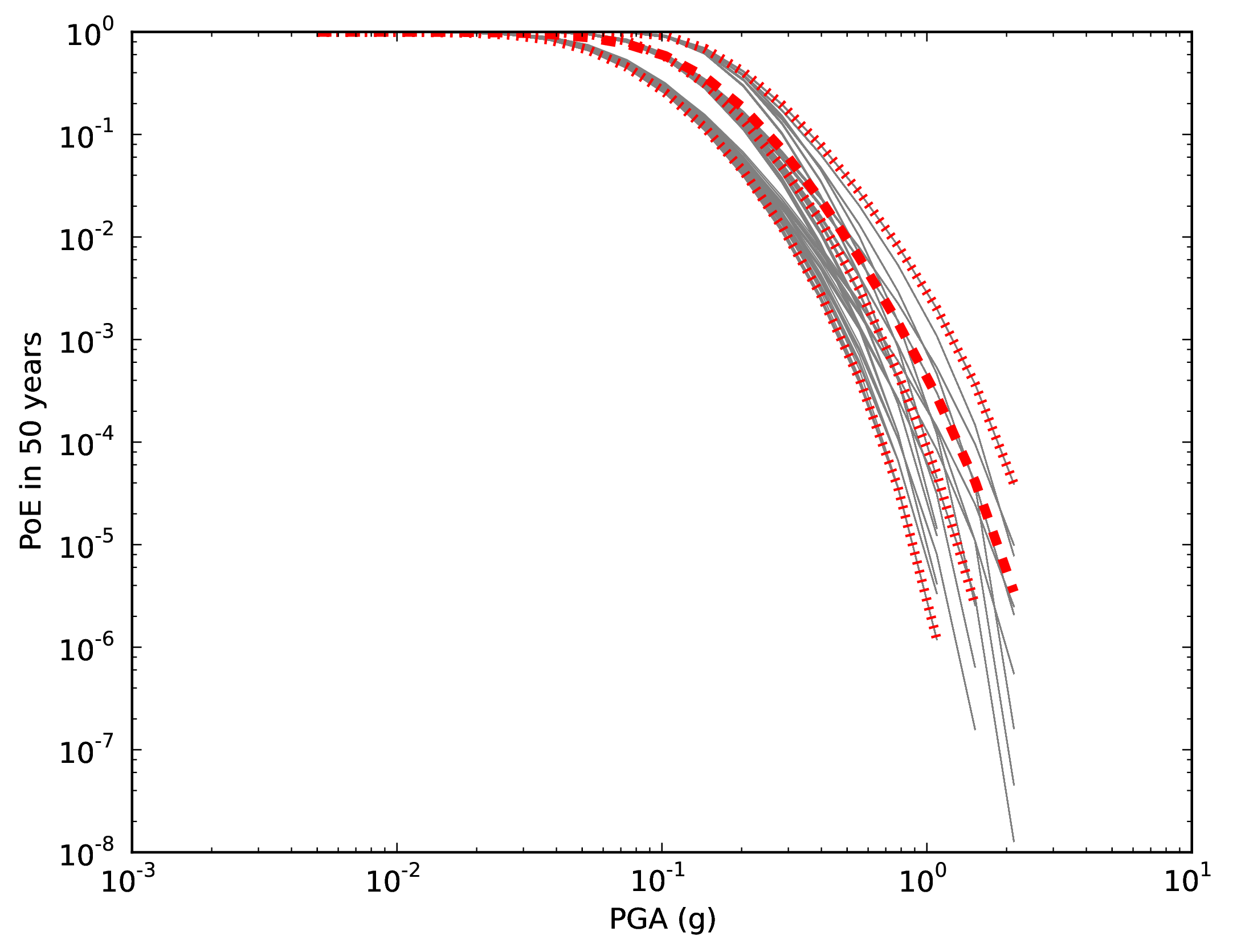
Fig. 2.18 Hazard curves as obtained from the LogicTreeCase2 demo. Solid gray lines represent individual hazard curves from the different logic tree path (a total of 324 curves). The red dashed line represents the mean hazard curve, while the red dotted lines depict the quantile levels (0.15, 0.5, 0.95).#
LogicTreeCase3ClassicalPSHA illustrates an example of logic tree defining relative uncertainties on G-R maximum magnitude and b value. A single source model is considered containing two sources belonging to different tectonic region types and both characterized by a G-R magnitude frequency distribution. The source model logic tree for this demo is as shown in the listing below.
 1<?xml version="1.0" encoding="UTF-8"?>
 2<nrml xmlns:gml="http://www.opengis.net/gml"
 3      xmlns="http://openquake.org/xmlns/nrml/0.5">
 4    <logicTree logicTreeID="lt1">
 5
 6            <logicTreeBranchSet uncertaintyType="sourceModel"
 7                                branchSetID="bs1">
 8                <logicTreeBranch branchID="b11">
 9                    <uncertaintyModel>
10                     source_model.xml
11                    </uncertaintyModel>
12                    <uncertaintyWeight>1.0</uncertaintyWeight>
13                </logicTreeBranch>
14            </logicTreeBranchSet>
15
16            <logicTreeBranchSet uncertaintyType="bGRRelative"
17                                branchSetID="bs21">
18                <logicTreeBranch branchID="b21">
19                    <uncertaintyModel>+0.1</uncertaintyModel>
20                    <uncertaintyWeight>0.333</uncertaintyWeight>
21                </logicTreeBranch>
22                <logicTreeBranch branchID="b22">
23                    <uncertaintyModel>0.0</uncertaintyModel>
24                    <uncertaintyWeight>0.333</uncertaintyWeight>
25                </logicTreeBranch>
26                <logicTreeBranch branchID="b23">
27                    <uncertaintyModel>-0.1</uncertaintyModel>
28                    <uncertaintyWeight>0.334</uncertaintyWeight>
29                </logicTreeBranch>
30            </logicTreeBranchSet>
31
32            <logicTreeBranchSet uncertaintyType="maxMagGRRelative"
33                                branchSetID="bs31">
34                <logicTreeBranch branchID="b31">
35                    <uncertaintyModel>0.0</uncertaintyModel>
36                    <uncertaintyWeight>0.333</uncertaintyWeight>
37                </logicTreeBranch>
38                <logicTreeBranch branchID="b32">
39                    <uncertaintyModel>+0.5</uncertaintyModel>
40                    <uncertaintyWeight>0.333</uncertaintyWeight>
41                </logicTreeBranch>
42                <logicTreeBranch branchID="b33">
43                    <uncertaintyModel>+1.0</uncertaintyModel>
44                    <uncertaintyWeight>0.334</uncertaintyWeight>
45                </logicTreeBranch>
46            </logicTreeBranchSet>
47
48    </logicTree>
49</nrml>
After the first branching level defining the source model, two
additional branching levels are defined, one defining relative
uncertainties on b value (bGRRelative applied consistently to all
sources in the source model) and the second uncertainties on maximum
magnitude (maxMagGRRelative). Similar to the other cases, two GMPEs
are considered for each tectonic region type and therefore the total
number of logic tree path is 36 (1 source model x 3 b value increments x
3 maximum magnitude increments x 2 GMPE for Active x 2 GMPEs for
Stable).
2.4.2. Hazard Disaggregation Demos#
An example of disaggregation calculation is given considering a source model consisting of two sources (area and simple fault) belonging to two different tectonic region types.
The calculation is defined with the following configuration file:
[general]
description = ...
calculation_mode = disaggregation
random_seed = 23

[geometry]
sites = 0.5 -0.5

[logic_tree]
number_of_logic_tree_samples = 0

[erf]
rupture_mesh_spacing = 2
width_of_mfd_bin = 0.1
area_source_discretization = 5.0

[site_params]
reference_vs30_type = measured
reference_vs30_value = 600.0
reference_depth_to_2pt5km_per_sec = 5.0
reference_depth_to_1pt0km_per_sec = 100.0

[calculation]
source_model_logic_tree_file = source_model_logic_tree.xml
gsim_logic_tree_file = gmpe_logic_tree.xml
investigation_time = 50.0
intensity_measure_types_and_levels = {"PGA": [...]}
truncation_level = 3
maximum_distance = 200.0

[disaggregation]
poes_disagg = 0.1
mag_bin_width = 1.0
distance_bin_width = 10.0
coordinate_bin_width = 0.2
num_epsilon_bins = 3

[output]
export_dir = ...
Disaggregation matrices are computed for a single site (located between
the two sources) for a ground motion value corresponding to a
probability value equal to 0.1 (poes_disagg = 0.1). Magnitude values
are classified in one magnitude unit bins (mag_bin_width = 1.0),
distances in bins of 10 km (distance_bin_width = 10.0), coordinates
in bins of 0.2 degrees (coordinate_bin_width = 0.2). 3 epsilons bins
are considered (num_epsilon_bins = 3).
2.4.3. Event Based PSHA Demos#
A demo showing an example of Event Based PSHA calculation is provided with the following configuration file:
[general]
description = Event Based PSHA using Area Source
calculation_mode = event_based
random_seed = 23

[geometry]
sites = 0.5 -0.5

[logic_tree]
number_of_logic_tree_samples = 0

[erf]
rupture_mesh_spacing = 2
width_of_mfd_bin = 0.1
area_source_discretization = 5.0

[site_params]
reference_vs30_type = measured
reference_vs30_value = 600.0
reference_depth_to_2pt5km_per_sec = 5.0
reference_depth_to_1pt0km_per_sec = 100.0

[calculation]
source_model_logic_tree_file = source_model_logic_tree.xml
gsim_logic_tree_file = gmpe_logic_tree.xml
investigation_time = 50.0
intensity_measure_types_and_levels = {"PGA": [...]}
truncation_level = 3
maximum_distance = 200.0

[event_based_params]
ses_per_logic_tree_path = 100
ground_motion_correlation_model =
ground_motion_correlation_params =

[output]
export_dir = ...
ground_motion_fields = true
hazard_curves_from_gmfs = true
mean = false
quantiles =
hazard_maps = true
poes = 0.1
The source model consist of one source (area). 100 stochastic event sets
are generated (ses_per_logic_tree_path = 100) (an example can be
seen in Fig. 2.19).
Ground motion fields are
computed (ground_motion_fields = true,
Fig. 2.20 and Fig. 2.21)
and also hazard curves from ground
motion fields are extracted (hazard_curves_from_gmfs = true). The
corresponding hazard maps for 0.1 probability are also calculated
(hazard_maps = true)
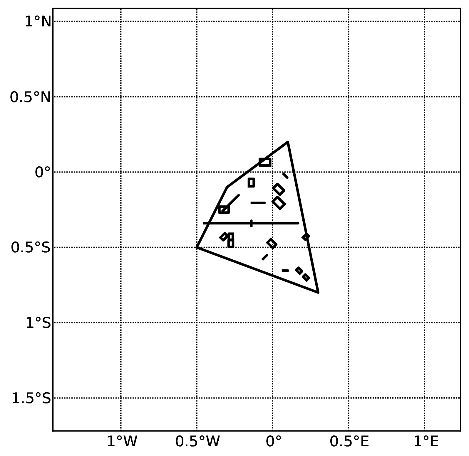
Fig. 2.19 A stochastic event set generated with the event based PSHA demo. The area source defines a nodal plane distribution which distributes events among vertical and dipping (50 degrees) faults with equal weights. Vertical ruptures are then distributed equally in the range 0-180 degrees while the dipping ones in the range 0-360, both with a step of 45 degrees.#
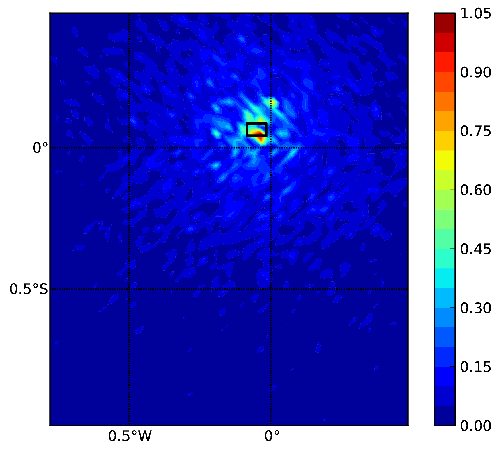
Fig. 2.20 Ground motion fields (PGA) with no spatial correlation#
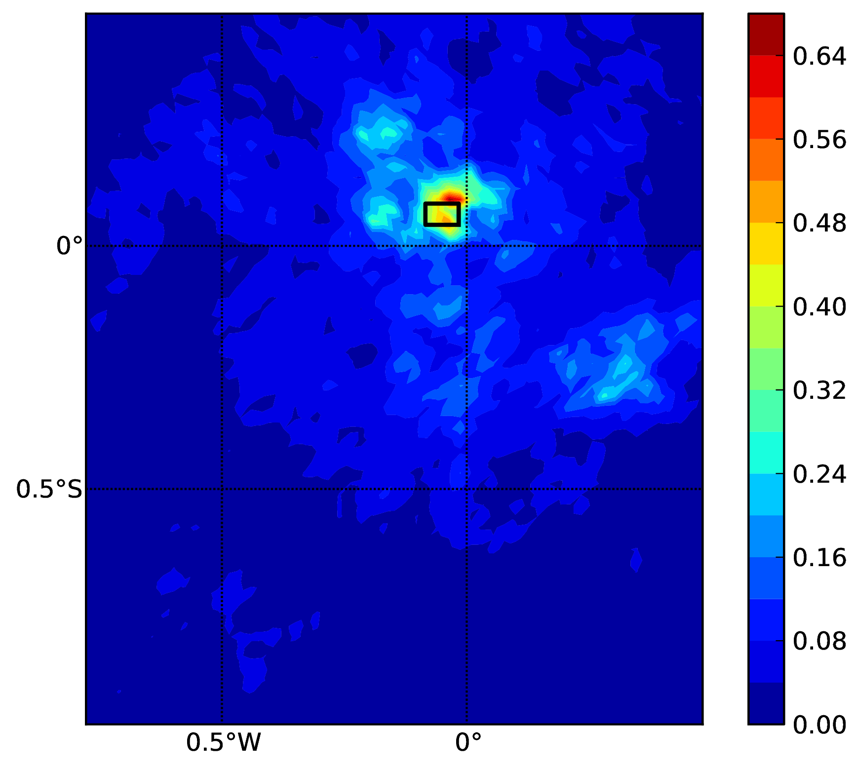
Fig. 2.21 Ground motion fields (PGA) with spatial correlation#