Cloud analysis fundamentals#
The cloud analysis proposed by Jalayer et al (2015) requires the definition of a best fit curve between an intensity measure (IM) and an engineering demand parameter (EDP) in the logarithmic space (see Figure 1).
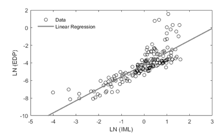
Figure. 1 Scatter of ln(EDP) and ln(IM), with the associated best-fit linear regression (adapted from Martins and Silva (2020)).
In numerical analyses convergence can be attained for levels of displacement that are incompatible with structural stability. This occurs mainly due to limitations in numerical modelling and it can introduce bias in the best-fit curve. In an effort to mitigate these effects a censored regression was implemented. Censored regression analysis requires the definition of a threshold (i.e. maximum displacement or acceleration) (see example in Figure 2), after which the data points are assumed to be affected by numerical errors. This threshold is defined by a censoring factor defined as the ratio between the maximum admissible EDP and the threshold for last damage state considered (e.g., complete damage). For example, a censoring factor equal to 1.5 means that EDPs 1.5 times above the threshold for the last damage state will be treated differently. A step-by-step description of this process can be found in Martins and Silva (2020).
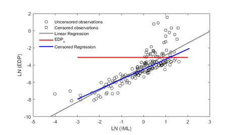
Figure. 2 Scatter of ln(EDP) and ln(IM), with the associated best-fit uncensored and censored regressions (adapted from Martins and Silva (2020)).
The expected EDP given an IM (E[ln(EDPi)]) and the respective uncertainty due to the record-to-record variability (σrec_to_rec) can be computed from the regression parameters (i.e. a and b) as follows
When building-to-building variability has not been explicitly considered (e.g. only one capacity curve has been provided per building class), it is possible to increase the uncertainty to account for this source of variability. To perform this adjustment one can add to the dispersion of the record-to-record variability (σrec_to_rec) the contribution of the building-to-building variability (σbld_to_bld). Gokkaya et al. (2016) and Casotto et al. (2015) recommend a value of 0.30 for this parameter.
The probability that a given damage state will be reached or exceeded given an intensity measure (P[DS≥dsi|IM]) can be computed from the equation below where EDPdsi stands for the engineering demand parameter (i.e. maximum displacement) for damage state dsi.
An example of computing a fragility function following the cloud analysis methodology can be found in Figure 3.
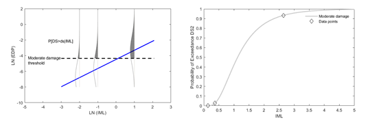
Figure. 3 Example of construction of a fragility function following the cloud analysis approach (adapted from Martins and Silva (2020))
References#
Casotto, C., Silva, V., Crowley, H., Nascimbene, R. and Pinho, R. (2015) Seismic fragility of Italian RC precast industrial structures. Engineering Structures, 94: p. 122-136. DOI: https://doi.org/10.1016/j.engstruct.2015.02.034
Gokkaya, B.U., Baker, J.W. and Deierlein, G.G. (2016) Quantifying the impacts of modeling uncertainties on the seismic drift demands and collapse risk of buildings with implications on seismic design checks. Earthquake Engineering & Structural Dynamics, 45(10): p. 1661-1683. DOI: https://doi.org/10.1002/eqe.2740
Jalayer, F., De Risi, R. and Manfredi, G. (2015) Bayesian Cloud Analysis: efficient structural fragility assessment using linear regression. Bulletin of Earthquake Engineering, 13(4): p. 1183-1203. DOI: 10.1007/s10518-014-9692-z.
Martins, L. and Silva, V. (2020) Development of a fragility and vulnerability model for global seismic risk analyses. Bulletin of Earthquake Engineering. DOI: 10.1007/s10518-020-00885-1.