14. Post-Earthquake Recovery Modelling Methodology

This work was supported by the State of California, Alfred E. Alquist Seismic Safety Commission and is part of a collaborative effort between the Global Earthquake Model (GEM) and the University of California at Los Angeles (UCLA), Department of Civil and Environmental Engineering. GEM implemented the scientific methodology developed by UCLA [BDL+15] and integrated it into the QGIS framework as part of the IRMT plugin.

This computational tool was developed to quantify the effectiveness of specific resilience-building actions (preparedness and response) that would enhance the process of recovery following an earthquake. Building performance is assessed using metrics that are explicitly linked to community seismic resilience such as functionality, occupiability and repairability. A probabilistic approach to mapping the fragility function parameters for the loss-based damage states used in OpenQuake and HAZUS (e.g. slight, moderate, extensive, complete) to the recovery-based damage states (e.g. functional loss, uninhabitable, irreparable) that are needed to assess seismic resilience is applied. A discrete state-based stochastic simulation model is used to quantify recovery trajectories for damaged buildings. Deterministic recovery paths conditioned on the post-earthquake damage state are described by discrete recovery states and the time spent in each state. The uncertainty in the recovery trajectory is captured by generating multiple realizations of the recovery path (Monte Carlo Simulation) accounting for the uncertainty in the time spent in each state. The function that describes community-level (or neighborhood-level) recovery is obtained by aggregating the recovery curves for the individual buildings after accounting for the variation in shaking and damage at each site and various exogenous and endogenous factors that affect the pace of recovery.

This tool provides an effective way to engage key stakeholders from government, industry and other groups, who are concerned with enhancing post-disaster recovery of communities. For example, focus groups with practitioners and emergency managers can be held to demonstrate its capabilities and explore their questions and concerns with regards to post-earthquake recovery. By allowing them to explore various trajectories for specific earthquake scenarios, the simulator will assist policy-makers, municipal governments and planners in understanding the possible interventions and tradeoffs associated with post-earthquake recovery. The simulation model can also be used to investigate hypotheses derived from findings and conclusions from previous earthquakes. Hypothesis examples include the following:

1. increased utility restoration rates increase recovery rates,
2. higher insurance penetration rates reduce household displacement,
3. designing for higher building performance levels prevents outmigration from the city, and
4. ‘residential red zones’ or temporary building moratoriums are preferable to patchwork reconstruction.

The recovery framework previously described was incorporated into this plugin, resulting in a dynamic and user-friendly software tool for generating both building-by-building and community level post-earthquake recovery predictions. The IRMT allows users to:

1. incorporate their local knowledge and data;
2. develop composite indicators (or indices) to measure social vulnerability and/or disaster resilience;
3. integrate these indices with physical risk estimates from OpenQuake or other software platforms; and
4. visualize the results.

In the following steps, a brief description of the basic workflow to develop an end-to-end recovery prediction is presented, where the main features and capabilities of the tool are highlighted.

14.1. Preparation of the input files for the OpenQuake Engine analysis

The recovery modelling algorithm requires users to provide a CSV file containing the probability of exceedance of each limit state for each individual building in the exposure model. The latter can be computed by running a Scenario Damage Assessment, which is a type of analysis supported by the risk component of the OpenQuake Engine. The input files necessary for running a scenario damage calculation and the resulting output files are depicted in Fig. 14.1 For technical details, definitions and examples of each component, readers are referred to [PMW+14] and [SCP+14].

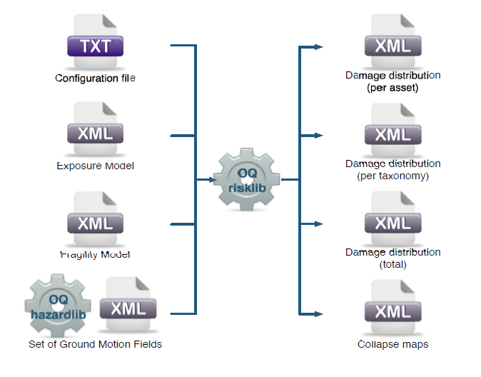
Fig. 14.1 Scenario Damage Calculator input/output structure

The window that requests users to upload the input files and run the scenario damage calculation is shown in Fig. 15.1.

It should be noted that in order to use the OpenQuake Engine from QGIS, the user needs to set up the connection with a working OpenQuake Engine Server using the IRMT settings dialog; the server can be installed in the same machine where the plugin is used. Alternatively, it is possible to use a remote server or cluster.

14.2. Setting up the configuration variables to run the recovery modelling algorithm

The configuration variables that are necessary to perform the recovery modeling analysis can be edited using the dialog shown in Fig. 14.2.

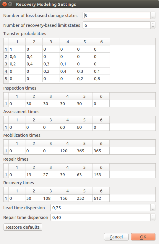
Fig. 14.2 Recovery modeling settings dialog

The following variables should be adjusted to the available data and needs of the user:

Configuration variable	Explanation
Number of loss-based damage states	Default is 5 (no damage, slight, moderate, extensive, complete)
Number of functional-based limit states	Default is 6 (no damage, trigger inspection, loss function, not occupiable, irreparable, collapse)
Transfer Probabilities	The element (i, j) of the matrix is the probability that the recovery-based limit state j occurs, given the loss-based damage state i
Assessment times	Time to conduct engineering assessment
Inspection times	Time to complete inspections
Mobilization times	Time to mobilize for construction
Recovery times	Period between the occurrence of the earthquake and the restoration of full functionality
Repair times	Time to replace elements in buildings or to reconstruct buildings
Repair times dispersion	Level of uncertainty associated with the repair times
Lead times dispersion	Level of uncertainty associated with the lead times

The list of the outputs from the Scenario Damage calculation can be visualized in Fig. 15.1. The tool offers the possibility to load the ‘Damage by asset’ CSV file (dmg_by_asset) as a QGIS vector layer, stored in the user’s computer as a shapefile. In addition, it is possible to automatically style the layer with respect to a chosen damage state. Alternatively, the user can upload on QGIS the ‘Damage by asset’ CSV file, structured in the same format as produced by the OpenQuake Engine. If the user does not need to edit the layer by adding or removing fields to/from it, it is possible to perform the recovery modelling calculation using the CSV-based layer. Otherwise, the layer should be converted and saved as a shapefile. Please note that shapefile limitations will reduce the field names to a maximum length of 10 characters each. At this point, the user may choose between two workflows on how to proceed to the generation of single buildings and/or community level recovery curves.

14.3. Interactive workflow

The user can select individual buildings (or a group of buildings) and the respective recovery curve (single or aggregated) is automatically developed. The curve can be edited, digitized and exported as a CSV, as well as saved as an image. The user requests the development of recovery curves by selecting the relevant layer, opening the IRMT Data Viewer (making sure that the Toggle viewer dock option is checked in the IRMT menu), and setting the Output Type tab to Recovery Curves. One of two available algorithmic approaches, regarding the estimation of the recovery, has to be chosen. The Aggregate approach produces the recovery model as a single process, whereas the Disaggregate approach takes into account four processes: inspection, assessment, mobilization and repair. In addition, the user can manually select the fields of the layer that contain the probabilities of being in each damage state (Fig. 16.3). If the file with the damage state probabilities is in the same format as produced by OpenQuake, the software pre-selects the appropriate fields for the recovery modelling algorithm. The number of simulations per building is the number of damage realizations used in Monte Carlo Simulation.

Warning

Increasing the number of simulations, the model becomes more accurate, but the calculation becomes slower and more expensive in terms of memory consumption

It should be emphasized that the integration of the recovery modelling algorithm in the QGIS software enables the users to adapt the workflow to their needs, leveraging all the features provided by the QGIS framework. The QGIS Processing Toolbox gives access to a wide variety of geoalgorithms, seamlessly integrating several different open-source resources, such as R, SAGA or GDAL. For instance, a SAGA algorithm, the ‘Add Polygon Attributes to Points’, can be used to aggregate by zone a set of selected assets, resulting in relating each asset to the identifier of the geographical area (zone) where it belongs. Following, the selection of the set of assets to be considered in the analysis can be performed in several different ways. The user can directly select points by clicking them on the map, or select points by using a formula. If points have been labeled with the identifier of the zone, the selection can be done with respect to the zone identification (or ID).

14.4. Batch workflow

Initially, the user must select the layer containing the information regarding the damage state probabilities per asset (see Preparation of the input files for the OpenQuake Engine analysis), after which the specific fields that contain these probabilities shall be opted. Next, the user must select a specific recovery time approach (Aggregate/Disaggregate) and set the number of simulations per building (number of damage realizations used in Monte Carlo Simulation). Here, it is possible to select the layer of the study area with zonal geometries and generate aggregated recovery curves by zones.

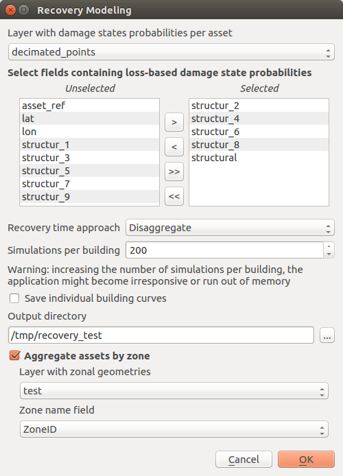
Fig. 14.3 Dialog to perform recovery modeling on the whole data set (also enabling zonal aggregation)

By unchecking the Aggregate assets by zone box (Fig. 14.3) the algorithm generates a single community recovery curve by aggregating the recovery curves of all the buildings within the region. The graphs, like the one shown in Fig. 14.4, are saved in the output directory designated by the user. In addition, building-by-building recovery curves are digitized and can be saved as text files (.txt) in the same output directory. The user can decide whether or not to generate the building-by-building recovery curves by (un)checking the Save individual building curves tab. The data can be further used (e.g. with a spreadsheet editor like LibreOffice Calc or Microsoft Excel) to generate and visualize individual building recovery curves that may be of interest to the user.

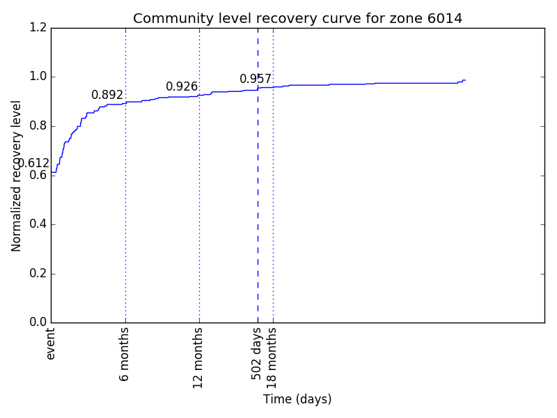
Fig. 14.4 The community-level recovery function for one of the zones under analysis, showing how the normalized recovery level evolves with time after the earthquake