13. Leveraging R to perform statistical analysis in QGIS
Socioeconomic analysis often involve statistical investigation, for instance for dimensionality reduction in problems involving a considerable number of variables. QGIS is well integrated with tools that can be leveraged for this kind of purpose. R is a well-known free software environment for statistical computing and graphics. It is widely used and easily installable on all the most used operating systems. QGIS enables users to drive R scripts from within the QGIS Processing Toolbox. This documentation explains how to make R scripts available in the Processing Toolbox. You can create your own scripts or download examples from a public repository. Scripts can be managed and edited directly within QGIS, through an embedded graphical widget. This feature is especially convenient to users who need to quickly customize existing scripts. However, it does not provide the same flexibility and interactivity that the R console offers, therefore the coding process becomes a little more challenging. By default, on unix-based systems, scripts are locally collected in the directory ~/.qgis2/processing/rscripts and they are identified by a file like scriptname.rsx, that contains the script itself, and an optional file like scriptname.rsx.help, that provides the corresponding documentation. An example taken from the above public repository is the following:
File Summary_statistics.rsx:
##Basic statistics=group
##Layer=vector
##Field=Field Layer
Summary_statistics<-data.frame(rbind(sum(Layer[[Field]]),
length(Layer[[Field]]),
length(unique(Layer[[Field]])),
min(Layer[[Field]]),
max(Layer[[Field]]),
max(Layer[[Field]])-min(Layer[[Field]]),
mean(Layer[[Field]]),
median(Layer[[Field]]),
sd(Layer[[Field]])),row.names=c("Sum:","Count:","Unique values:","Minimum value:","Maximum value:","Range:","Mean value:","Median value:","Standard deviation:"))
colnames(Summary_statistics)<-c(Field)
>Summary_statistics
File Summary_statistics.rsx.help:
{"ALG_DESC": "This tool calculates the following summary statistics for a
              numeric field: (1) Sum, (2) Count, (3) Unique values,
              (4) Minimum value, (5) Maximum value, (6) Range, (7) Mean,
              (8) Median and (9) Standard deviation.\n\n",
"R_CONSOLE_OUTPUT": "Summary statistics table",
"ALG_CREATOR": "Filipe S. Dias, filipesdias(at)gmail.com",
"Layer": "Input vector with at least one numeric field",
"Field": "Numeric field",
"ALG_HELP_CREATOR": "Filipe S. Dias, filipesdias(at)gmail.com"}
Note that the header of the script contains some lines beginning with ##. These lines are used by the QGIS Processing Toolkit to build a graphical user interface that will be displayed every time the script is launched, and that enables users to graphically set up some parameters that will be used by the script. In the example, for instance, a dropdown menu will list all the available vector layers; once a layer is selected, another dropdown menu will list all its fields. Please refer to the QGIS documentation for a more detailed description of the script syntax.
A brief list of statistical techniques that are often needed in socioeconomic analysis, that are all available in R, are as follows:
- Summary statistics (mean, median, high value, low value, standard deviation)
- Boxplots as well as measures of skewness and curtosis
- Histograms
- Scatter plotting
- Correlation (Pearson’s R, Spearman Rank, Kendall’s Tau)
- Cronbach’s Alpha (which is based on correlation)
- Principal Components Analysis/Factor Analysis
Some of these require the statistical platform to take into account one single field (e.g., summary statistics) or a couple of fields (e.g. scatterplot). In such cases, it is sufficient to add parametric references to those fields into the header of the script. Things become more complicated where the number of parameters required is not known in advance, as in the case of Principal Components Analysis. Unfortunately, at the time of writing, the widgets that can be used through the script header syntax do not include a multiselection functionality, such as this). Therefore, it is impossible for the user to graphically select an indefinite number of fields from the complete list. What we can do, however, is to let our script perform the analysis on the whole set of numeric fields available in the selected layer. In case we want to exclude some numeric fields from the analysis, we can add to the script header the reference to a textual field to be added to the GUI, in which the user can insert a list of comma-separated names of fields to be ignored. The script becomes something like:
##Basic statistics=group
##Layer=vector
##Exclude=String
layerData <- data.frame(Layer)
numericFields <- sapply(layerData, is.numeric)
numericData <- layerData[, numericFields]
excludedFields <- trimws(strsplit(Exclude, ",")[[1]])
analyzedData <- numericData[, !(names(numericData) %in% excludedFields)]
comps <- prcomp(analyzedData, scale=TRUE)
>comps
What if we want to build a vector layer using the results of a calculation performed by R? Examples of this are available in the documentation linked above. The following example shows how to load a vector layer from those available in QGIS, make a copy of it, perform a calculation, save the result in a new field of the new layer, and make the final layer available in QGIS. In this basic example, the calculation is extremely simple, just summing the values of two fields. However, it can be easily extended to obtain complex results.
##Vector processing=group
##Layer=vector
##First=Field Layer
##Second=Field Layer
##output=output vector
modified <- data.frame(Layer)
modified['SUM'] <- NA
modified$SUM <- Layer[[First]] + Layer[[Second]]
output=SpatialPolygonsDataFrame(Layer, as.data.frame(modified))
We have just seen in the latter example that the output of a script can be a vector layer (##output=output vector). In the previous example, >comps indicated to the Processing Toolkit that the object comps had to be shown to the user as text in a dedicated output window. A third possibility is to display the output as a plot, using the ##showplots directive as follows:
##Vector processing=group
##showplots
##Layer=vector
##Field=Field Layer
##Unit=String
boxplot(Layer[[Field]], main="BOXPLOT", xlab=paste(Field), ylab=paste(Unit))
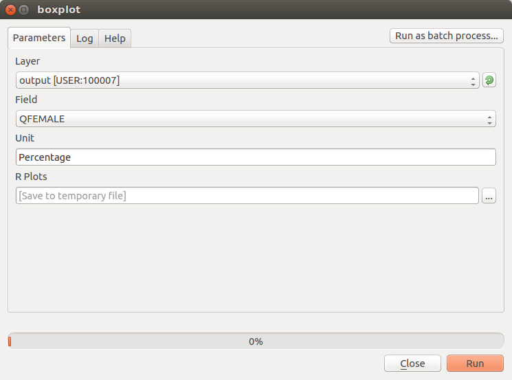
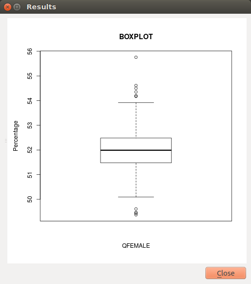
When the script is executed, the dialog shown in Fig. 13.1 allows the user select one of the available layers, then one of its fields. In the Unit text field, the user can write the measurement unit to be displayed in the y label in the plot. By pressing Run, R is started, running the boxplot function on the selected data and setting the plot labels accordingly (see Fig. 13.2).

