9. Weighting data and calculating indices

Fig. 9.1 Tree chart structure for the development of composite indicators

Central to the construction of composite indicators is the need to meaningfully combine different data dimensions, and consideration must be given to weighting and aggregation procedures. Most composite indicators rely on equal weighting largely for simplicity. Equal weighting, however, implies that all variables within the composite indicator are of equal importance when this may not actually be the case. The issue of aggregation is similar to the weighting process. Different aggregation rules may be applied depending on the underlying theoretical framework chosen by the user for the modelling process. Sub-indicators may be summed up (linear aggregation) for instance, multiplied, or geometrically aggregated to correct for compensability (i.e., the possibility of offsetting a deficit in some dimension with an outstanding performance in another). Each technique has specific consequences, implies different assumptions, and could ignore or incorporate weights.

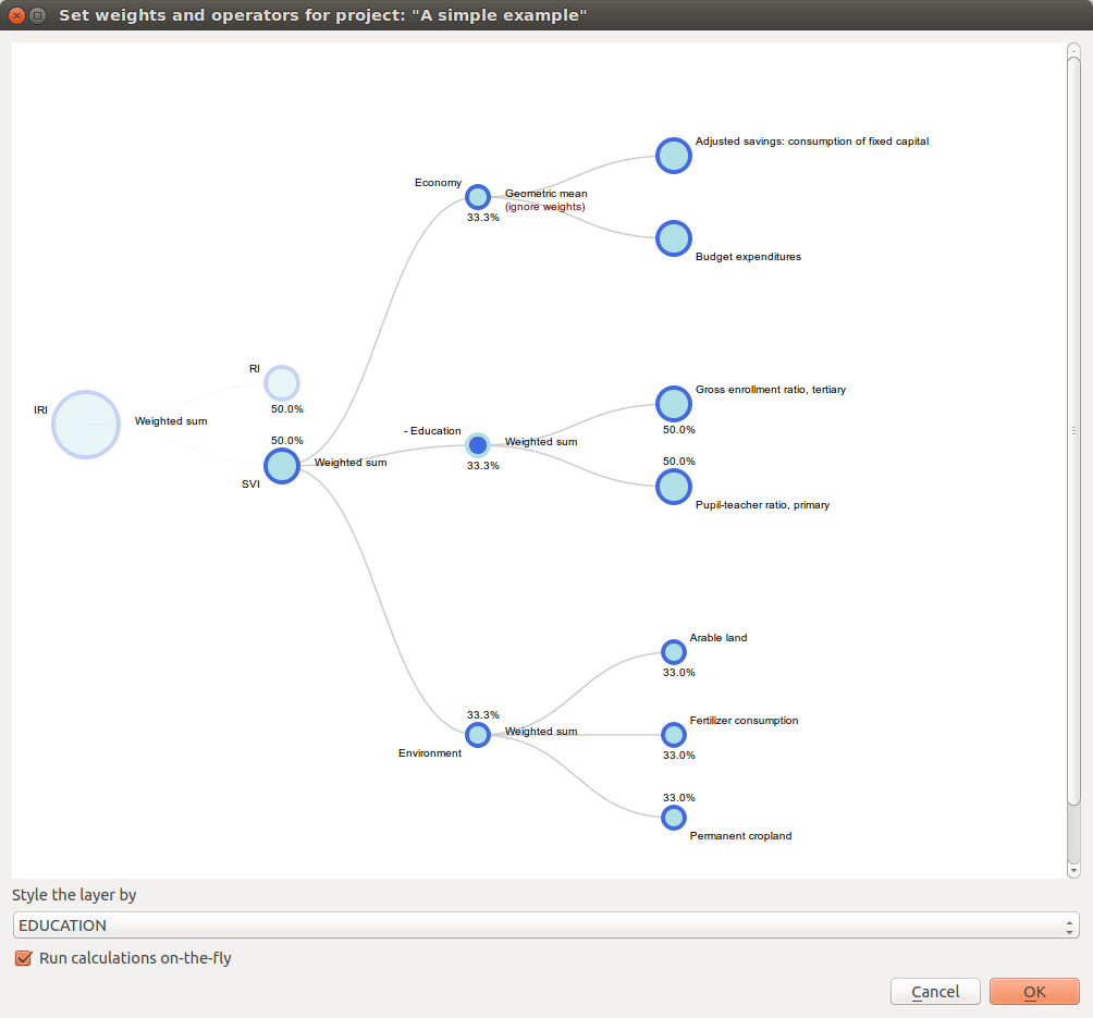
The Weight data and calculate indices widget (Fig. 9.1) is the key module of the IMRT. It contains the model building functionality of the IRMT, and it is used to create, edit, and manage composite indicator(s) and integrated risk model development. It provides users with an intuitive way to develop composite models by building and editing the selected project definition through the use of a dynamic graphical interface that was developed explicitly to guide the construction of composite indicators in a manner that is simple, visual, and straight-forward. The latter is accomplished through a window that embeds a dynamic model builder that takes the form of a tree chart (see Fig. 9.1). This structure (or weighting and aggregation tree) defines a workflow that strings together sequences of steps to describe how variables are combined together to obtain the composite indices.

Fig. 9.2 Composite indicator types

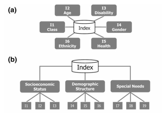
Currently, the IRMT supports the development of two composite model types: a) deductive and, b) hierarchical (Fig. 9.2 [1]). Deductive models typically contain fewer than ten indicators that are normalized and aggregated to create an index. Hierarchical models typically employ ten to twenty indicators that are separated into groups (sub-indices) that share the same underlying dimension of a concept (in this case socio-economic parameters of earthquake risk such as population, economy, infrastructure, education, and governance). Individual indicators are aggregated into sub-indices (e.g., population, economy, etc.), and the sub-indices are aggregated to form a final composite index (e.g., social vulnerability or integrated risk index). The tree structure of the Weight data and calculate indices widget encourages the development of hierarchical models of integrated risk. The starting point is a root node that corresponds to the development of a hierarchical model that can be: 1) an Integrated Risk Index (IRI) which is a function of the aggregation of a Social Vulnerability Index (SVI) and a Risk Index (RI); or 2) a Social Vulnerability Index (SVI) that is the result of the aggregation of various sub-indicators defined by the user (e.g., Economy, Education, and Environment as shown within Fig. 9.1).  The tree can be modified dynamically by adding or removing nodes, inverting variables, setting a weight to each variable or node and choosing the operators to be used to combine variables together.

Whenever Update or Update and close are clicked, the project definition is updated and the composite indices are re-calculated. As a consequence, the map is rendered and styled accordingly. This allows the user to have an immediate feedback on how the map changes depending on how the project definition is set. Such automatic re-calculations and rendering can take some time, depending on the complexity of the project and number of enumeration units analysed. Sometimes it is more convenient to disable the on-the-fly calculations while changing the project’s structure, and enable it again once the project has been built. In order to do so, it is sufficient to toggle the Run calculations on-the-fly checkbox.

The main functional elements of the weighting and aggregation tree are discussed in the subsections below.

9.1. Adding a node

Individual nodes correspond to aggregated composite indicators within the weighting and aggregation tree. To add a node (i.e., a composite sub-indicator) within the tree, it is possible to begin by left-clicking on the default node (i.e., SVI). Clicking on the default SVI node allows the addition of multiple new sub-indicators, each with its own user-provided name.

Note

It is not possible to add nodes stemming from the IRI.

When a newly created node is clicked, a new dialog is initiated to give users the option to select the variables available in the layer (and not already used in the node) to populate the sub-indicator being under construction.

Note

The SVI can be calculated if each socioeconomic sub-indicator has at least one variable.

In order to add an indicator to one of the socioeconomic sub-indicators, you can click on the corresponding node. When adding an indicator to the RI, or to one of the socioeconomic sub-indicators, the description of the node will be automatically set to be equal to the name of the corresponding layer’s variable. Users can edit this description, however, by clicking on the text displayed next to the node in the tree and then by clicking within the corresponding textbox to change the text.

9.2. Removing a node

In order to remove one of the nodes from the tree, users can perform a right-click on that node. A popup dialog window will ask you to confirm if you really intend to delete the node and all of its children (the lower level nodes connected to it).

Note

Removing a node from the tree will not delete the corresponding field from the layer.

9.3. Setting the operators to be used to aggregate variables

On the right of each node, the tree indicates the name of the operator to be used to combine (or aggregate) the variables making up the node. By clicking on the operator’s name, a dialog to set weights and operators is opened. The same happens when clicking on the name of one of the children nodes. The operator can be chosen from a dropdown menu. Some operators (e.g., Weighted sum) take into account the weights applied to the child nodes. Other operators (e.g., Average (ignore weights)) do not take into account weights. When the chosen operator is one of the latter, the child nodes will be rendered on the graphical display all with the same radius and their weights will not be rendered (see Fig. 9.1 for a demonstration of how the radius of nodes corresponds with the respective weights of variables). Otherwise, the radius of a node is proportional to its weight, and the weight is rendered next to the node.

9.4. Setting weights

Central to the construction of composite indicators in the need to combine data which implies decisions on weighting. The dialog to set weights is opened in the same way as described in Setting the operators to be used to aggregate variables. Several weighting techniques are available, and some make use of statistical models. For the IRMT we implemented a simple solution to weighting that is often based on the results of participatory approaches. A weight can be edited manually by clicking on its value and overwriting it with a new value. A weight can also be edited by clicking on the spinner’s arrows to increase or decrease the weight. By clicking Update, the weights will be re-calculated in order to make them sum to 1. In other words, if you have 3 variables and you set their weights to 1, 2 and 5 and you press Update, the weights will be re-calculated to be respectively 0.125, 0.250 and 0.625, keeping the same proportion between each other, and summing to 1.

9.5. Inverting a variable

The dialog to invert variables is opened in the same way as described in Setting the operators to be used to aggregate variables. If a variable contributes in a negative way to the composite indicator (e.g., a higher education corresponding to a lower social vulnerability), it is possible to indicate such an inverse relationship by pressing the Invert button next to the variable name. The effect on a composite indicator in response to this decision process and setting is that each value of an inverted variable will be to multiplied by -1 each time the variable is used in a calculation.

Note

Please note that the layer’s field will keep holding the original value of the variable, and that the inversion will be performed on-the-fly for the purpose of the calculation.

9.6. Assigning a new name to a variable

The dialog to assign a new name to a variable is also opened in the same way as described in Setting the operators to be used to aggregate variables. By clicking on the variable’s name, a popup dialog asks users to insert the new name. The project definition will be updated accordingly, linking the layer’s fieldname with the modified description.

9.7. Styling the layer by a chosen field

The dropdown menu entitled Style layer by on the bottom of the Set weights and operators module can be used to choose fields within a layer, i.e., fields other than those delineated within the project definition to be symbolized, allowing all fields in a layer to be to be symbolized on-the-fly. This can be useful, for instance, to map the values calculated for different sub-indicators, or even individual variables if they are of interest. By default, the selection is blank. In the default case, the tool will adopt the following convention: 1) if the IRI can be computed, then the layer will be symbolized according to it; 2) otherwise, if the SVI can be computed, then it will be used as the default case for symbolization in the absence of IRI; 3) otherwise, the convention will apply with respect to the RI; and 4) if none of main sub-indicators can be calculated, then the layer will not be re-styled unless the user uses the dropdown menu to specify a specific symbolization field.

[1]	Adapted from [TAT12]

[TAT12]

Tate, E.C. 2012. Social vulnerability indices: a comparative assessment using uncertainty and sensitivity analysis, Natural Hazards, 63(2): 325-347