Event Based

Scenario risk calculations usually do not pose a performance problem, since they involve a single rupture and a limited geography for analysis. Some event-based risk calculations, however, may involve millions of ruptures and exposures spanning entire countries or even larger regions. This section offers some practical tips for running large event based risk calculations, especially ones involving large logic trees, and proposes techniques that might be used to make an intractable calculation tractable.

Understanding the hazard

Event-based calculations are typically dominated by the hazard component (unless there are lots of assets aggregated on few hazard sites) and therefore the first thing to do is to estimate the size of the hazard, i.e. the number of GMFs that will be produced. Since we are talking about a large calculation, first of all we need reduce it to a size that is guaranteed to run quickly. The simplest way to do that is to reduce the parameters directly affecting the number of ruptures generated, i.e.

• investigation_time

• ses_per_logic_tree_path

• number_of_logic_tree_samples

For instance, if you have ses_per_logic_tree_path = 10,000 reduce it to 10, run the calculation and you will see in the log something like this:

[2018-12-16 09:09:57,689 #35263 INFO] Received
{'gmfdata': '752.18 MB', 'hcurves': '224 B', 'indices': '29.42 MB'}

The amount of GMFs generated for the reduced calculation is 752.18 MB; and since the calculation has been reduced by a factor of 1,000, the full computation is likely to generate around 750 GB of GMFs. Even if you have sufficient disk space to store this large quantity of GMFs, most likely you will run out of memory. Even if the hazard part of the calculation manages to run to completion, the risk part of the calculation is very likely to fail — managing 750 GB of GMFs is beyond the current capabilities of the engine. Thus, you will have to find ways to reduce the size of the computation.

A good start would be to carefully set the parameters minimum_magnitude and minimum_intensity:

• minimum_magnitude is a scalar or a dictionary keyed by tectonic region; the engine will discard ruptures with magnitudes below the given threshoulds

• minimum_intensity is a scalar or a dictionary keyed by the intensity measure type; the engine will discard GMFs below the given intensity threshoulds

Choosing reasonable cutoff thresholds with these parameters can significantly reduce the size of your computation when there are a large number of small magnitude ruptures or low intensity GMFs being generated, which may have a negligible impact on the damage or losses, and thus could be safely discarded.

region_grid_spacing

In our experience, the most common error made by out users is to compute the hazard at the sites of the exposure. The issue is that it very possible to have exposures with millions of assets on millions of distinct hazard sites. Computing the GMFs for millions of sites is hard or even impossible (there is a limit of 4 billion rows on the size of the GMF table in the datastore). Even in the cases when computing the hazard is possible, then computing the risk starting from an extremely large amount of GMFs will likely be impossible, due to memory/runtime constraints.

The second most common error is to use an extremely fine grid for the site model. Remember that if you have a resolution of 250 meters, a square of 250 km x 250 km will contain one million sites, which is definitely too much. The engine when designed when the site models had resolutions around 5-10 km, i.e. of the same order of the hazard grid, while nowadays the vs30 fields have a much larger resolution.

Both problems can be solved in a simple way by specifying the region_grid_spacing parameter. Make it large enough that the resulting number of sites becomes reasonable and you are done. You will loose some precision, but that is preferable to not being able to run the calculation. You will need to run a sensitivity analysis with different values of region_grid_spacing parameter to make sure that you get consistent results, but that’s it.

Once a region_grid_spacing is specified, the engine computes the convex hull of the exposure sites and builds a grid of hazard sites, associating the site parameters from the closest site in the site model and discarding sites in region where there are no assets (i.e. more distant than region_grid_spacing * sqrt(2)). The precise logic is encoded in the function openquake.commonlib.readinput.get_sitecol_assetcol, if you want to know the nitty-gritty details.

Our recommendation is to use the command oq prepare_site_model to apply such logic before starting a calculation and thus producing a custom site model file tailored to your exposure (see the section prepare_site_model).

Collapsing of branches

When one is not interested in the uncertainty around the loss estimates and cares more about the mean estimates, all of the source model branches can be “collapsed” into one branch. Using the collapsed source model should yield the same mean hazard or loss estimates as using the full source model logic tree and then computing the weighted mean of the individual branch results.

Similarly, the GMPE logic tree for each tectonic region can also be “collapsed” into a single branch. Using a single collapsed GMPE for each TRT should also yield the same mean hazard estimates as using the full GMPE logic tree and then computing the weighted mean of the individual branch results. This has become possible through the introduction of AvgGMPE feature in version 3.9.

Using collect_rlzs=true in the risk calculation

Since version 3.12 the engine recognizes a flag collect_rlzs in the risk configuration file, which by default is false. When the flag is set to true, then the hazard realizations are collected together when computing the risk results and considered as one. This is possible only when the weights of the realizations are all equal, otherwise the engine raises an error. Collecting the realizations makes the calculation of the losses and loss curves much faster and more memory efficient. It is the recommended way to proceed when you are interested only in mean results.

Note 1: when using sampling, collect_rlzs is implicitly set to True, so if you want to export the individual results per realization you must set explictly collect_rlzs=false.

Note 2: collect_rlzs is not the inverse of the individual rlsz flag. The two flags are completely independent, one refers to risk and the other to hazard calculations.

Note 3: collect_rlzs is completely ignored in the hazard part of the calculation, i.e. it does not affect at all the computation of the GMFs, only the computation of the risk curves.

Splitting the calculation into subregions

If one is interested in propagating the full uncertainty in the source models or ground motion models to the hazard or loss estimates, collapsing the logic trees into a single branch to reduce computational expense is not an option. But before going through the effort of trimming the logic trees, there is an interim step that must be explored, at least for large regions like the entire continental United States. This step is to geographically divide the large region into logical smaller subregions, such that the contribution to the hazard or losses in one subregion from the other subregions is negligibly small or even zero. The effective realizations in each of the subregions will then be much fewer than when trying to cover the entire large region in a single calculation.

Trimming of the logic-trees or sampling of the branches

Trimming or sampling may be necessary if the following two conditions hold:

1. You are interested in propagating the full uncertainty to the hazard and loss estimates; only the mean or quantile results are not sufficient for your analysis requirements, AND

2. The region of interest cannot be logically divided further as described above; the logic-tree for your chosen region of interest still leads to a very large number of effective realizations.

Sampling is the easier of the two options now. You only need to ensure that you sample a sufficient number of branches to capture the underlying distribution of the hazard or loss results you are interested in. The drawback of random sampling is that you may still need to sample hundreds of branches to capture well the underlying distribution of the results.

Trimming can be much more efficient than sampling, because you pick a few branches such that the distribution of the hazard or loss results obtained from a full-enumeration of these branches is nearly the same as the distribution of the hazard or loss results obtained from a full-enumeration of the entire logic-tree.

ignore_covs vs ignore_master_seed

The vulnerability functions using continuous distributions (lognormal/beta) to characterize the uncertainty in the loss ratio, specify the mean loss ratios and the corresponding coefficients of variation for a set of intensity levels.

There is clearly a performance/memory penalty associated with the propagation of uncertainty in the vulnerability to losses. You can completely remove it by setting

ignore_covs = true

in the job.ini file. Then the engine would compute just the mean loss ratios by ignoring the uncertainty i.e. the coefficients of variation. Since engine 3.12 there is a better solution: setting

ignore_master_seed = true

in the job.ini file. Then the engine will compute the mean loss ratios but also store information about the uncertainty of the results in the asset loss table, in the column “variance”, by using the formulae

\[\begin{split}variance &= \Sigma_i \sigma_i^2 \ for\ asset\_correl=0 \\ variance &= (\Sigma_i \sigma_i)^2 \ for\ asset\_correl=1\end{split}\]

in terms of the variance of each asset for the event and intensity level in consideration, extracted from the asset loss and the coefficients of variation. People interested in the details should look at the implementation in gem/oq-engine.

The asset loss table

When performing an event based risk calculation the engine keeps in memory a table with the losses for each asset and each event, for each loss type. It is usually impossible to fully store such table, because it is extremely large; for instance, for 1 million assets, 1 million events, 2 loss types and 4 bytes per loss ~8 TB of disk space would be required. It is true that many events will produce zero losses because of the maximum_distance and minimum_intensity parameters, but still the asset loss table is prohibitively large and for many years could not be stored. In engine 3.8 we made a breakthrough: we decided to store a partial asset loss table, obtained by discarding small losses, by leveraging on the fact that loss curves for long enough return periods are dominated by extreme events, i.e. there is no point in saving all the small losses.

To that aim,the engine honors a parameter called minimum_asset_loss which determine how many losses are discarded when storing the asset loss table. The rule is simple: losses below minimum_asset_loss are discarded. By choosing the threshold properly in an ideal world

1. the vast majority of the losses would be discarded, thus making the asset loss table storable;

2. the loss curves would still be nearly identical to the ones without discarding any loss, except for small return periods.

It is the job of the user to verify if 1 and 2 are true in the real world. He can assess that by playing with the minimum_asset_loss in a small calculation, finding a good value for it, and then extending to the large calculation. Clearly it is a matter of compromise: by sacrificing precision it is possible to reduce enourmously the size of the stored asset loss table and to make an impossible calculation possible.

Starting from engine 3.11 the asset loss table is stored if the user specifies

aggregate_by = id

in the job.ini file. In large calculations it extremely easy to run out of memory or the make the calculation extremely slow, so we recommend not to store the asset loss table. The functionality is there for the sole purpose of debugging small calculations, for instance to see the effect of the minimum_asset_loss approximation at the asset level.

For large calculations usually one is interested in the aggregate loss table, which contains the losses per event and per aggregation tag (or multi-tag). For instance, the tag occupancy has the three values “Residential”, “Industrial” and “Commercial” and by setting

aggregate_by = occupancy

the engine will store a pandas DataFrame called risk_by_event with a field agg_id with 4 possible value: 0 for “Residential”, 1 for “Industrial”, 2 for “Commercial” and 3 for the full aggregation.

NB: if the parameter aggregate_by is not specified, the engine will still compute the aggregate loss table but then the agg_id field will have a single value 0 corresponding to the total portfolio losses.

The Probable Maximum Loss (PML) and the loss curves

Given an effective investigation time and a return period, the engine is able to compute a PML for each aggregation tag. It does so by using the function openquake.risklib.scientific.losses_by_period which takes in input an array of cumulative losses associated to the aggregation tag, a list of or return periods, and the effective investigation time. If there is a single return period the function returns the PML; if there are multiple return periods it returns the loss curve. The two concepts are essentially the same thing, since a loss curve is just an array of PMLs, one for each return period. For instance

>>> from openquake.risklib.scientific import losses_by_period
>>> losses = [3, 2, 3.5, 4, 3, 23, 11, 2, 1, 4, 5, 7, 8, 9, 13, 0]
>>> [PML_500y] = losses_by_period(losses, [500], eff_time=1000)
>>> PML_500y
13.0

computes the Probably Maximum Loss at 500 years for the given losses with an effective investigation time of 1000 years. The algorithm works by ordering the losses (suppose there are E > 1 losses) generating E time periods eff_time/E, eff_time/(E-1), ... eff_time/1 and log-interpolating the loss at the return period. Of course this works only if the condition

eff_time/E < return_period < eff_time

is respected. In this example there are E=16 losses, so the return period must be in the range 62.5 .. 1000 years. If the return period is too small the PML will be zero

>>> losses_by_period(losses, [50], eff_time=1000)
array([0.])

while if the return period is outside the investigation range we will refuse the temptation to extrapolate and we will return NaN instead:

>>> losses_by_period(losses, [1500], eff_time=1000)
array([nan])

The rules above are the reason while you will see zeros or NaNs in the loss curves generated by the engine sometimes, especially when there are too few events: the valid range will be small and some return periods may slip outside the range.

In order to compute aggregate loss curves you must set the aggregate_by parameter in the job.ini to one or more tags over which you wish to perform the aggregation. Your exposure must contain the specified tags with values for each asset. We have an example for Nepal in our event based risk demo. The exposure for this demo contains various tags and in particular a geographic tag called NAME1 with values “Mid-Western”, “Far-Western”, “West”, “East”, “Central”, and the job_eb.ini file defines

aggregate_by = NAME_1

When running the calculation you will see something like this:

 Calculation 1 finished correctly in 17 seconds
id | name
 9 | Aggregate Event Losses
 1 | Aggregate Loss Curves
 2 | Aggregate Loss Curves Statistics
 3 | Aggregate Losses
 4 | Aggregate Losses Statistics
 5 | Average Asset Losses Statistics
11 | Earthquake Ruptures
 6 | Events
 7 | Full Report
 8 | Input Files
10 | Realizations
12 | Total Loss Curves
13 | Total Loss Curves Statistics
14 | Total Losses
15 | Total Losses Statistics

Exporting the Aggregate Loss Curves Statistics output will give you the mean and quantile loss curves in a format like the following one:

annual_frequency_of_exceedence,return_period,loss_type,loss_value,loss_ratio
5.00000E-01,2,nonstructural,0.00000E+00,0.00000E+00
5.00000E-01,2,structural,0.00000E+00,0.00000E+00
2.00000E-01,5,nonstructural,0.00000E+00,0.00000E+00
2.00000E-01,5,structural,0.00000E+00,0.00000E+00
1.00000E-01,10,nonstructural,0.00000E+00,0.00000E+00
1.00000E-01,10,structural,0.00000E+00,0.00000E+00
5.00000E-02,20,nonstructural,0.00000E+00,0.00000E+00
5.00000E-02,20,structural,0.00000E+00,0.00000E+00
2.00000E-02,50,nonstructural,0.00000E+00,0.00000E+00
2.00000E-02,50,structural,0.00000E+00,0.00000E+00
1.00000E-02,100,nonstructural,0.00000E+00,0.00000E+00
1.00000E-02,100,structural,0.00000E+00,0.00000E+00
5.00000E-03,200,nonstructural,1.35279E+05,1.26664E-06
5.00000E-03,200,structural,2.36901E+05,9.02027E-03
2.00000E-03,500,nonstructural,1.74918E+06,1.63779E-05
2.00000E-03,500,structural,2.99670E+06,1.14103E-01
1.00000E-03,1000,nonstructural,6.92401E+06,6.48308E-05
1.00000E-03,1000,structural,1.15148E+07,4.38439E-01

If you do not set the aggregate_by parameter you will still able to compute the total loss curve (for the entire portfolio of assets), and the total average losses.

Aggregating by multiple tags

The engine also supports aggregation my multiple tags. For instance the second event based risk demo (the file job_eb.ini) has a line

aggregate_by = NAME_1, taxonomy

and it is able to aggregate both on geographic region (NAME_1) and on taxonomy. There are 25 possible combinations, that you can see with the command:

$ oq show agg_keys
| NAME_1_ | taxonomy_ | NAME_1      | taxonomy                   |
+---------+-----------+-------------+----------------------------+
| 1       | 1         | Mid-Western | Wood                       |
| 1       | 2         | Mid-Western | Adobe                      |
| 1       | 3         | Mid-Western | Stone-Masonry              |
| 1       | 4         | Mid-Western | Unreinforced-Brick-Masonry |
| 1       | 5         | Mid-Western | Concrete                   |
| 2       | 1         | Far-Western | Wood                       |
| 2       | 2         | Far-Western | Adobe                      |
| 2       | 3         | Far-Western | Stone-Masonry              |
| 2       | 4         | Far-Western | Unreinforced-Brick-Masonry |
| 2       | 5         | Far-Western | Concrete                   |
| 3       | 1         | West        | Wood                       |
| 3       | 2         | West        | Adobe                      |
| 3       | 3         | West        | Stone-Masonry              |
| 3       | 4         | West        | Unreinforced-Brick-Masonry |
| 3       | 5         | West        | Concrete                   |
| 4       | 1         | East        | Wood                       |
| 4       | 2         | East        | Adobe                      |
| 4       | 3         | East        | Stone-Masonry              |
| 4       | 4         | East        | Unreinforced-Brick-Masonry |
| 4       | 5         | East        | Concrete                   |
| 5       | 1         | Central     | Wood                       |
| 5       | 2         | Central     | Adobe                      |
| 5       | 3         | Central     | Stone-Masonry              |
| 5       | 4         | Central     | Unreinforced-Brick-Masonry |
| 5       | 5         | Central     | Concrete                   |

The lines in this table are associated to the generalized aggregation ID, agg_id which is an index going from 0 (meaning aggregate assets with NAME_1=*Mid-Western* and taxonomy=*Wood*) to 24 (meaning aggregate assets with NAME_1=*Mid-Western* and taxonomy=*Wood*); moreover agg_id=25 means full aggregation.

The agg_id field enters in risk_by_event and in outputs like the aggregate losses; for instance:

$ oq show agg_losses-rlzs
| agg_id | rlz | loss_type     | value       |
+--------+-----+---------------+-------------+
| 0      | 0   | nonstructural | 2_327_008   |
| 0      | 0   | structural    | 937_852     |
+--------+-----+---------------+-------------+
| ...    + ... + ...           + ...         +
+--------+-----+---------------+-------------+
| 25     | 1   | nonstructural | 100_199_448 |
| 25     | 1   | structural    | 157_885_648 |

The exporter (oq export agg_losses-rlzs) converts back the agg_id to the proper combination of tags; agg_id=25, i.e. full aggregation, is replaced with the string *total*.

By knowing the number of events, the number of aggregation keys and the number of loss types, it is possible to give an upper limit to the size of risk_by_event. In the demo there are 1703 events, 26 aggregation keys and 2 loss types, so risk_by_event contains at most

1703 * 26 * 2 = 88,556 rows

This is an upper limit, since some combination can produce zero losses and are not stored, especially if the minimum_asset_loss feature is used. In the case of the demo actually only 20,877 rows are nonzero:

$ oq show risk_by_event
       event_id  agg_id  loss_id           loss      variance
...
[20877 rows x 5 columns]

Rupture sampling: how does it work?

In this section we explain how the sampling of ruptures in event based calculations works, at least for the case of Poissonian sources. As an example, consider the following point source:

>>> from openquake.hazardlib import nrml
>>> src = nrml.get('''\
... <pointSource id="1" name="Point Source"
...              tectonicRegion="Active Shallow Crust">
...     <pointGeometry>
...         <gml:Point><gml:pos>179.5 0</gml:pos></gml:Point>
...         <upperSeismoDepth>0</upperSeismoDepth>
...         <lowerSeismoDepth>10</lowerSeismoDepth>
...     </pointGeometry>
...     <magScaleRel>WC1994</magScaleRel>
...     <ruptAspectRatio>1.5</ruptAspectRatio>
...     <truncGutenbergRichterMFD aValue="3" bValue="1" minMag="5" maxMag="7"/>
...     <nodalPlaneDist>
...         <nodalPlane dip="30" probability="1" strike="45" rake="90" />
...     </nodalPlaneDist>
...     <hypoDepthDist>
...         <hypoDepth depth="4" probability="1"/>
...     </hypoDepthDist>
... </pointSource>''', investigation_time=1, width_of_mfd_bin=1.0)

The source here is particularly simple, with only one seismogenic depth and one nodal plane. It generates two ruptures, because with a width_of_mfd_bin of 1 there are only two magnitudes in the range from 5 to 7:

>>> [(mag1, rate1), (mag2, rate2)] = src.get_annual_occurrence_rates()
>>> mag1
5.5
>>> mag2
6.5

The occurrence rates are respectively 0.009 and 0.0009. So, if we set the number of stochastic event sets to 1,000,000

>>> num_ses = 1_000_000

we would expect the first rupture (the one with magnitude 5.5) to occur around 9,000 times and the second rupture (the one with magnitude 6.5) to occur around 900 times. Clearly the exact numbers will depend on the stochastic seed; if we set

>>> import numpy.random
>>> numpy.random.seed(42)

then we will have (for investigation_time = 1)

>>> numpy.random.poisson(rate1 * num_ses * 1)
8966
>>> numpy.random.poisson(rate2 * num_ses * 1)
921

These are the number of occurrences of each rupture in the effective investigation time, i.e. the investigation time multiplied by the number of stochastic event sets and the number of realizations (here we assumed 1 realization).

The total number of events generated by the source will be

number_of_events = sum(n_occ for each rupture)

i.e. 8,966 + 921 = 9,887, with ~91% of the events associated to the first rupture and ~9% of the events associated to the second rupture.

Since the details of the seed algorithm can change with updates to the the engine, if you run an event based calculation with the same parameters with different versions of the engine, you may not get exactly the same number of events, but something close given a reasonably long effective investigation time. After running the calculation, inside the datastore, in the ruptures dataset you will find the two ruptures, their occurrence rates and their integer number of occurrences (n_occ). If the effective investigation time is large enough the relation

n_occ ~ occurrence_rate * eff_investigation_time

will hold. If the effective investigation time is not large enough, or the occurrence rate is extremely small, then you should expect to see larger differences between the expected number of occurrences and n_occ, as well as a strong seed dependency.

It is important to notice than in order to determine the effective investigation time, the engine takes into account also the ground motion logic tree and the correct formula to use is

eff_investigation_time = investigation_time * num_ses * num_rlzs

where num_rlzs is the number of realizations in the ground motion logic tree.

Just to be concrete, if you run a calculation with the same parameters as described before, but with two GMPEs instead of one (and number_of_logic_tree_samples = 0), then the total number of paths admitted by the logic tree will be 2 and you should expect to get about twice the number of occurrences for each rupture. Users wanting to know the nitty-gritty details should look at the code, inside hazardlib/source/base.py, in the method src.sample_ruptures(eff_num_ses, ses_seed).

The case of multiple tectonic region types and realizations

Since engine 3.13 hazardlib contains some helper functions that allow users to compute stochastic event sets manually. Such functions are in the module openquake.hazardlib.calc.stochastic. Internally, the engine does not use directly such functions, since it needs to follow a slightly more complex logic in order to make the calculations parallelizable. Also, the engine is able to manage general source model logic trees, while the helper functions are meant to work in a situation with a single source model and a trivial source model logic tree. However, in spirit, the idea is the same.

As a concrete example, consider the event based logic tree demo which is part of the engine distribution (search for demos/hazard/EventBasedPSHA). This is a case with a trivial source model logic tree, a source model with two tectonic region types and a GSIM logic tree generating 2x2 = 4 realizations with weights .36, .24, .24, .16 respectively. The effective investigation time is

eff_time = 50 years x 250 ses x 4 rlz = 50,000 years

You can sample the ruptures with the following commands, assuming you are inside the demo directory:

>> from openquake.hazardlib.contexts import ContextMaker
>> from openquake.commonlib import readinput
>> from openquake.hazardlib.calc.stochastic import sample_ebruptures
>> oq = readinput.get_oqparam('job.ini')
>> gsim_lt = readinput.get_gsim_lt(oq)
>> csm = readinput.get_composite_source_model(oq)
>> rlzs_by_gsim_trt = gsim_lt.get_rlzs_by_gsim_trt(
..     oq.number_of_logic_tree_samples, oq.random_seed)
>> cmakerdict = {trt: ContextMaker(trt, rbg, vars(oq))
..                    for trt, rbg in rlzs_by_gsim_trt.items()}
>> ebruptures = sample_ebruptures(csm.src_groups, cmakerdict)

Then you can extract the events associated to the ruptures with the function get_ebr_df which returns a DataFrame:

>> from openquake.hazardlib.calc.stochastic import get_ebr_df
>> ebr_df = get_ebr_df(ebruptures, cmakerdict)

This DataFrame has fields eid (event ID) and rlz (realization number) and it is indexed by the ordinal of the rupture. For instance it can be used to determine the number of events per realization:

>> ebr_df.groupby('rlz').count()
eid   rlz
0    7842
1    7709
2    7893
3    7856

Notice that the number of events is more or less the same for each realization. This is a general fact, valid also in the case of sampling, a consequence of the random algorithm used to associate the events to the realizations.

The difference between full enumeration and sampling

Users are often confused about the difference between full enumeration and sampling. For this reason the engine distribution comes with a pedagogical example that considers an extremely simplified situation comprising a single site, a single rupture, and only two GMPEs. You can find the example in the engine repository under the directory openquake/qa_tests_data/event_based/case_3. If you look at the ground motion logic tree file, the two GMPEs are AkkarBommer2010 (with weight 0.9) and SadighEtAl1997 (with weight 0.1).

The parameters in the job.ini are:

investigation_time = 1
ses_per_logic_tree_path = 5_000
number_of_logic_tree_paths = 0

Since there are 2 realizations, the effective investigation time is 10,000 years. If you run the calculation, you will generate (at least with version 3.13 of the engine, though the details may change with the version) 10,121 events, since the occurrence rate of the rupture was chosen to be 1. Roughly half of the events will be associated with the first GMPE (AkkarBommer2010) and half with the second GMPE (SadighEtAl1997). Actually, if you look at the test, the precise numbers will be 5,191 and 4,930 events, i.e. 51% and 49% rather than 50% and 50%, but this is expected and by increasing the investigation time you can get closer to the ideal equipartition. Therefore, even if the AkkarBommer2010 GMPE is assigned a relative weight that is 9 times greater than SadighEtAl1997, this is not reflected in the simulated event set. It means that when performing a computation (for instance to compute the mean ground motion field, or the average loss) one has to keep the two realizations distinct, and only at the end to perform the weighted average.

The situation is the opposite when sampling is used. In order to get the same effective investigation time of 10,000 years you should change the parameters in the job.ini to:

investigation_time = 1
ses_per_logic_tree_path = 1
number_of_logic_tree_paths = 10_000

Now there are 10,000 realizations, not 2, and they all have the same weight .0001. The number of events per realization is still roughly constant (around 1) and there are still 10,121 events, however now the original weights are reflected in the event set. In particular there are 9,130 events associated to the AkkarBommer2010 GMPE and 991 events associated to the SadighEtAl1997 GMPE. There is no need to keep the realizations separated: since they have all the same weigths, you can trivially compute average quantities. AkkarBommer2010 will count more than SadighEtAl1997 simply because there are 9 times more events for it (actually 9130/991 = 9.2, but the rate will tend to 9 when the effective time will tend to infinity).

NB: just to be clear, normally realizations are not in one-to-one correspondence with GMPEs. In this example, it is true because there is a single tectonic region type. However, usually there are multiple tectonic region types, and a realization is associated to a tuple of GMPEs.

Extra tips specific to event based calculations

Event based calculations differ from classical calculations because they produce visible ruptures, which can be exported and made accessible to the user. In classical calculations, instead, the underlying ruptures only live in memory and are normally not saved in the datastore, nor are exportable. The limitation is fundamentally a technical one: in the case of an event based calculation only a small fraction of the ruptures contained in a source are actually generated, so it is possible to store them. In a classical calculation all ruptures are generated and there are so many millions of them that it is impractical to save them, unless there are very few sites. For this reason they live in memory, they are used to produce the hazard curves and immediately discarded right after. The exception if for the case of few sites, i.e. if the number of sites is less than the parameter max_sites_disagg which by default is 10.

Sampling of the logic tree

There are real life examples of very large logic trees, like the model for South Africa which features 3,194,799,993,706,229,268,480 branches. In such situations it is impossible to perform a computation with full enumeration. However, the engine allows to sample the branches of the complete logic tree. More precisely, for each branch sampled from the source model logic tree, a branch of the GMPE logic tree is chosen randomly, by taking into account the weights in the GMPE logic tree file.

It should be noticed that even if source model path is sampled several times, the model is parsed and sent to the workers only once. In particular if there is a single source model (like for South America) and number_of_logic_tree_samples =100, we generate effectively 1 source model realization and not 100 equivalent source model realizations, as we did in past (actually in the engine version 1.3). The engine keeps track of how many times a model has been sampled (say Ns) and in the event based case it produce ruptures (with different seeds) by calling the appropriate hazardlib function Ns times. This is done inside the worker nodes. In the classical case, all the ruptures are identical and there are no seeds, so the computation is done only once, in an efficient way.

Convergency of the GMFs for non-trivial logic trees

In theory, the hazard curves produced by an event based calculation should converge to the curves produced by an equivalent classical calculation. In practice, if the parameters number_of_logic_tree_samples and ses_per_logic_tree_path (the product of them is the relevant one) are not large enough they may be different. The engine is able to compare the mean hazard curves and to see how well they converge. This is done automatically if the option mean_hazard_curves = true is set. Here is an example of how to generate and plot the curves for one of our QA tests (a case with bad convergence was chosen on purpose):

$ oq engine --run event_based/case_7/job.ini
<snip>
WARNING:root:Relative difference with the classical mean curves for IMT=SA(0.1): 51%
WARNING:root:Relative difference with the classical mean curves for IMT=PGA: 49%
<snip>
$ oq plot /tmp/cl/hazard.pik /tmp/hazard.pik --sites=0,1,2

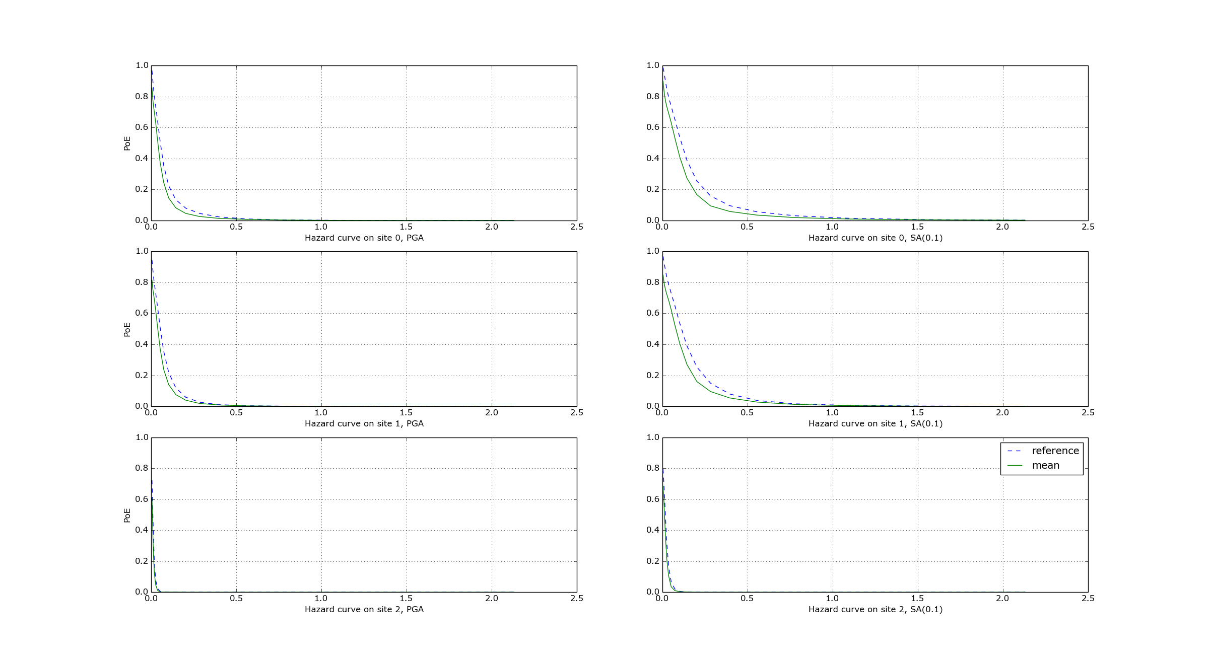
The relative difference between the classical and event based curves is computed by computing the relative difference between each point of the curves for each curve, and by taking the maximum, at least for probabilities of exceedence larger than 1% (for low values of the probability the convergency may be bad). For the details I suggest you to look at the code.

The concept of “mean” ground motion field

The engine has at least three different kinds of mean ground motion field, computed differently and used in different situations:

1. Mean ground motion field by GMPE, used to reduce disk space and make risk calculations faster.

2. Mean ground motion field by event, used for debugging/plotting purposes.

3. Single-rupture hazardlib mean ground motion field, used for analysis/plotting purposes.

Mean ground motion field by GMPE

This is the most useful concept for people doing risk calculations. To be concrete, suppose you are running a scenario_risk calculation on a region where you have a very fine site model (say at 1 km resolution) and a sophisticated hazard model (say with 16 different GMPEs): then you can easily end up with a pretty large calculation. For instance one of our users was doing such a calculation with an exposure of 1.2 million assets, 50,000+ hazard sites, 5 intensity measure levels and 1000 simulations, corresponding to 16,000 events given that there are 16 GMPEs. Given that each ground motion value needs 4 bytes to be stored as a 32 bit float, the math tells us that such calculation will generate 50000 x 16000 x 5 x 4 ~ 15 GB of data (it could be a but less by using the minimum_intensity feature, but you get the order of magnitude). This is very little for the engine that can store such an amount of data in less than 1 minute, but it is a huge amount of data for a database. If you a (re)insurance company and your workflow requires ingesting the GMFs in a database to compute the financial losses, that’s a big issue. The engine could compute the hazard in just an hour, but the risk part could easily take 8 days. This is a no-go for most companies. They have deadlines and cannot way 8 days to perform a single analysis. At the end they are interested only in the mean losses, so they would like to have a single effective mean field producing something close to the mean losses that more correctly would be obtained by considering all 16 realizations. With a single effective realization the data storage would drop under 1 GB and more significantly the financial model software would complete the calculation in 12 hours instead of 8 days, something a lot more reasonable.

For this kind of situations hazardlib provides an AvgGMPE class, that allows to replace a set of GMPEs with a single effective GMPE. More specifically, the method AvgGMPE.get_means_and_stddevs calls the methods .get_means_and_stddevs on the underlying GMPEs and performs a weighted average of the means and a weighted average of the variances using the usual formulas:

\[\begin{split}\mu &= \Sigma_i w_i \mu_i \\ \sigma^2 &= \Sigma_i w_i (\sigma_i)^2\end{split}\]

where the weights sum up to 1. It is up to the user to check how big is the difference in the risk between the complete calculation and the mean field calculation. A factor of 2 discrepancies would not be surprising, but we have also seen situations where there is no difference within the uncertainty due to the random seed choice.

Mean ground motion field by event

Using the AvgGMPE trick does not solve the issue of visualizing the ground motion fields, since for each site there are still 1000 events. A plotting tool has still to download 1 GB of data and then one has to decide which event to plot. The situation is the same if you are doing a sensitivity analysis, i.e. you are changing some parameter (it could be a parameter of the underlying rupture, or even the random seed) and you are studying how the ground motion fields change. It is hard to compare two sets of data of 1 GB each. Instead, it is a lot easier to define a “mean” ground motion field obtained by averaging on the events and then compare the mean fields of the two calculations: if they are very different, it is clear that the calculation is very sensitive to the parameter being studied. Still, the tool performing the comparison will need to consider 1000 times less data and will be 1000 times faster, also downloding 1000 times less data from the remote server where the calculation has been performed.

For this kind of analysis the engine provides an internal output avg_gmf that can be plotted with the command oq plot avg_gmf <calc_id>. It is also possible to compare two calculations with the command

$ oq compare avg_gmf imt <calc1> <calc2>

Since avg_gmf is meant for internal usage and for debugging it is not exported by default and it is not visible in the WebUI. It is also not guaranteed to stay the same across engine versions. It is available starting from version 3.11. It should be noted that, consistently with how the AvgGMPE works, the avg_gmf output is computed in log space, i.e. it is geometric mean, not the usual mean. If the distribution was exactly lognormal that would also coincide with the median field.

However, you should remember that in order to reduce the data transfer and to save disk space the engine discards ground motion values below a certain minimum intensity, determined explicitly by the user or inferred from the vulnerability functions when performing a risk calculation: there is no point in considering ground motion values below the minimum in the vulnerability functions, since they would generate zero losses. Discarding the values below the threshould breaks the log normal distribution.

To be concrete, consider a case with a single site, and single intensity measure type (PGA) and a minimum_intensity of 0.05g. Suppose there are 1000 simulations and that you have a normal distribution of the logaritms with \(\mu\)sigma`=.5; then the ground motion values that you could obtain would be as follows:

>>> import numpy
>>> numpy.random.seed(42) # fix the seed
>>> gmvs = numpy.random.lognormal(mean=-2.0, sigma=.5, size=1000)

As expected, the variability of the values is rather large, spanning more than one order of magnitude:

>>> gmvs.min(), numpy.median(gmvs), gmvs.max()
(0.026765710489091852, 0.1370582013790309, 0.9290114132955762)

Also mean and standard deviation of the logarithms are very close to the expected values \(\mu\)sigma`=.5:

>>> numpy.log(gmvs).mean()
-1.9903339720888376
>>> numpy.log(gmvs).std()
0.4893631038736771

The geometric mean of the values (i.e. the exponential of the mean of the logarithms) is very close to the median, as expected for a lognormal distribution:

>>> numpy.exp(numpy.log(gmvs).mean())
0.13664978061122787

All these properties are broken when the ground motion values are truncated below the minimum_intensity:

>> gmvs[gmvs < .05] = .05
>> numpy.log(gmvs).mean()

-1.9876078473466177 >> numpy.log(gmvs).std() 0.48280630467779523 >> numpy.exp(numpy.log(gmvs).mean()) 0.13702281319482504

In this case the difference is minor, but if the number of simulations is small and/or the \(\sigma\) is large the mean and standard deviation obtained from the logarithms of the ground motion fields could be quite different from the expected ones.

Finally, it should be noticed that the geometric mean can be orders of magnitude different from the usual mean and it is purely a coincidence that in this case they are close (~0.137 vs ~0.155).

Single-rupture estimated median ground motion field

The mean ground motion field by event discussed above is an a posteriori output: after performing the calculation, some statistics are performed on the stored ground motion fields. However, in the case of a single rupture it is possible to estimate the geometric mean and the geometric standard deviation a priori, using hazardlib and without performing a full calculation. However, there are some limitations to this approach:

1. it only works when there is a single rupture

2. you have to manage the minimum_intensity manually if you want to compare with a concrete engine output

3. it is good for estimates, it gives you the theoretical ground ground motion field but not the ones concretely generated by the engine fixed a specific seed

It should also be noticed that there is a shortcut to compute the single-rupture hazardlib “mean” ground motion field without writing any code; just set in your job.ini the following values:

truncation_level = 0
ground_motion_fields = 1

Setting truncation_level = 0 effectively replaces the lognormal distribution with a delta function, so the generated ground motion fields will be all equal, with the same value for all events: this is why you can set ground_motion_fields = 1, since you would just waste time and space by generating multiple copies.

Finally let’s warn again on the term hazardlib “mean” ground motion field: in log space it is truly a mean, but in terms of the original GMFs it is a geometric mean - which is the same as the median since the distribution is lognormal - so you can also call this the hazardlib median ground motion field.

How the hazard sites are determined

There are several ways to specify the hazard sites in an engine calculation.

1. The user can specify the sites directly in the job.ini using the sites parameter (e.g. sites = -122.4194 37.7749, -118.2437 34.0522, -117.1611 32.7157). This method is perhaps most useful when the analysis is limited to a handful of sites.

2. Otherwise the user can specify the list of sites in a CSV file (i.e. sites_csv = sites.csv).

3. Otherwise the user can specify a grid via the region and region_grid_spacing parameters.

4. Otherwise the sites can be inferred from the exposure, if any, in two different ways:

   1. if region_grid_spacing is specified, a grid is implicitly generated from the convex hull of the exposure and used

   2. otherwise the locations of the assets are used as hazard sites

5. Otherwise the sites can be inferred from the site model file, if any.

It must be noted that the engine rounds longitudes and latitudes to 5 decimal places (or approximately 1 meter spatial resolution), so sites that differ only at the 6th decimal place or beyond will end up being considered as duplicated sites by the engine, and this will be flagged as an error.

Having determined the sites, a SiteCollection object is generated by associating the closest parameters from the site model (if any) or using the global site parameters, if any. If the site model is specified, but the closest site parameters are too distant from the sites, a warning is logged for each site.

There are a number of error situations:

1. If both site model and global site parameters are missing, the engine raises an error.

2. If both site model and global site parameters are specified, the engine raises an error.

3. Specifying both the sites.csv and a grid is an error.

4. Specifying both the sites.csv and a site_model.csv is an error. If you are in such situation you should consider using the command oq prepare_site_model to manually prepare a site model on the location of the sites.

5. Having duplicates (i.e. rows with identical lon, lat up to 5 digits) in the site model is an error.

If you want to compute the hazard on the locations specified by the site model and not on the exposure locations, you can split the calculation in two files: job_haz.ini containing the site model and job_risk.ini containing the exposure. Then the risk calculator will find the closest hazard to each asset and use it. However, if the closest hazard is more distant than the asset_hazard_distance parameter (default 15 km) an error is raised.

Scenarios from ShakeMaps

Beginning with version 3.1, the engine is able to perform scenario_risk and scenario_damage calculations starting from the GeoJSON feed for ShakeMaps provided by the United States Geological Survey (USGS). Furthermore, starting from version 3.12 it is possible to use ShakeMaps from other sources like the local filesystem or a custom URL.

Running the Calculation

In order to enable this functionality one has to prepare a parent calculation containing the exposure and risk functions for the region of interest, say Peru. To that aim the user will need to write a prepare_job.ini file like this one:

[general]
description = Peru - Preloading exposure and vulnerability
calculation_mode = scenario
exposure_file = exposure_model.xml
structural_vulnerability_file = structural_vulnerability_model.xml

By running the calculation

$ oq engine --run prepare_job.ini

The exposure and the risk functions will be imported in the datastore.

This example only includes vulnerability functions for the loss type structural, but one could also have in this preparatory job file the functions for nonstructural components and contents, and occupants, or fragility functions if damage calculations are of interest.

It is essential that each fragility/vulnerability function in the risk model should be conditioned on one of the intensity measure types that are supported by the ShakeMap service – MMI, PGV, PGA, SA(0.3), SA(1.0), and SA(3.0). If your fragility/vulnerability functions involves an intensity measure type which is not supported by the ShakeMap system (for instance SA(0.6)) the calculation will terminate with an error.

Let’s suppose that the calculation ID of this ‘pre’ calculation is 1000. We can now run the risk calculation starting from a ShakeMap. For that, one need a job.ini file like the following:

[general]
description = Peru - 2007 M8.0 Pisco earthquake losses
calculation_mode = scenario_risk
number_of_ground_motion_fields = 10
truncation_level = 3
shakemap_id = usp000fjta
spatial_correlation = yes
cross_correlation = yes

This example refers to the 2007 Mw8.0 Pisco earthquake in Peru (see https://earthquake.usgs.gov/earthquakes/eventpage/usp000fjta#shakemap). The risk can be computed by running the risk job file against the prepared calculation:

$ oq engine --run job.ini --hc 1000

Starting from version 3.12 it is also possible to specify the following sources instead of a shakemap_id:

# (1) from local files:
shakemap_uri = {
      "kind": "usgs_xml",
      "grid_url": "relative/path/file.xml",
      "uncertainty_url": "relative/path/file.xml"
      }

# (2) from remote files:
shakemap_uri = {
      "kind": "usgs_xml",
      "grid_url": "https://url.to/grid.xml",
      "uncertainty_url": "https://url.to/uncertainty.zip"
      }

# (3) both files in a single archive
# containing grid.xml, uncertainty.xml:
shakemap_uri = {
      "kind": "usgs_xml",
      "grid_url": "relative/path/grid.zip"
      }

While it is also possible to define absolute paths, it is advised not to do so since using absolute paths will make your calculation not portable across different machines.

The files must be valid .xml USGS ShakeMaps (1). One or both files can also be passed as .zip archives containing a single valid xml ShakeMap (2). If both files are in the same .zip, the archived files must be named grid.xml and uncertainty.xml.

Also starting from version 3.12 it is possible to use ESRI Shapefiles in the same manner as ShakeMaps. Polygons define areas with the same intensity levels and assets/sites will be associated to a polygon if contained by the latter. Sites outside of a polygon will be discarded. Shapefile inputs can be specified similar to ShakeMaps:

shakemap_uri = {
   "kind": "shapefile",
   "fname": "path_to/file.shp"
}

It is only necessary to specify one of the available files, and the rest of the files will be expected to be in the same location. It is also possible to have them contained together in a *.zip file. There are at least a *.shp-main file and a *.dbf-dBASE file required. The record field names, intensity measure types and units all need to be the same as with regular USGS ShakeMaps.

Irrespective of the input, the engine will perform the following operations:

1. download the ShakeMap and convert it into a format suitable for further processing, i.e. a ShakeMaps array with lon, lat fields

2. the ShakeMap array will be associated to the hazard sites in the region covered by the ShakeMap

3. by using the parameters truncation_level and number_of_ground_motion_fields a set of ground motion fields (GMFs) following the truncated Gaussian distribution will be generated and stored in the datastore

4. a regular risk calculation will be performed by using such GMFs and the assets within the region covered by the shakemap.

Correlation

By default the engine tries to compute both the spatial correlation and the cross correlation between different intensity measure types. Please note that if you are using MMI as intensity measure type in your vulnerability model, it is not possible to apply correlations since those are based on physical measures.

For each kind of correlation you have three choices, that you can set in the job.ini, for a total of nine combinations:

- spatial_correlation = yes, cross_correlation = yes  # the default
- spatial_correlation = no, cross_correlation = no   # disable everything
- spatial_correlation = yes, cross_correlation = no
- spatial_correlation = no, cross_correlation = yes
- spatial_correlation = full, cross_correlation = full
- spatial_correlation = yes, cross_correlation = full
- spatial_correlation = no, cross_correlation = full
- spatial_correlation = full, cross_correlation = no
- spatial_correlation = full, cross_correlation = yes

yes means using the correlation matrix of the Silva-Horspool paper; no mean using no correlation; full means using an all-ones correlation matrix.

Apart from performance considerations, disabling either the spatial correlation or the cross correlation (or both) might be useful to see how significant the effect of the correlation is on the damage/loss estimates.

In particular, due to numeric errors, the spatial correlation matrix - that by construction contains only positive numbers - can still produce small negative eigenvalues (of the order of -1E-15) and the calculation fails with an error message saying that the correlation matrix is not positive defined. Welcome to the world of floating point approximation! Rather than magically discarding negative eigenvalues the engine raises an error and the user has two choices: either disable the spatial correlation or reduce the number of sites because that can make the numerical instability go away. The easiest way to reduce the number of sites is setting a region_grid_spacing parameter in the prepare_job.ini file, then the engine will automatically put the assets on a grid. The larger the grid spacing, the fewer the number of points, and the closer the calculation will be to tractability.

Performance Considerations

The performance of the calculation will be crucially determined by the number of hazard sites. For instance, in the case of the Pisco earthquake the ShakeMap has 506,142 sites, which is a significantly large number of sites. However, the extent of the ShakeMap in longitude and latitude is about 6 degrees, with a step of 10 km the grid contains around 65 x 65 sites; most of the sites are without assets because most of the grid is on the sea or on high mountains, so actually there are around ~500 effective sites. Computing a correlation matrix of size 500 x 500 is feasible, so the risk computation can be performed.

Clearly in situations in which the number of hazard sites is too large, approximations will have to be made such as using a larger region_grid_spacing. Disabling spatial AND cross correlation makes it possible run much larger calculations. The performance can be further increased by not using a truncation_level.

When applying correlation, a soft cap on the size of the calculations is defined. This is done and modifiable through the parameter cholesky_limit which refers to the number of sites multiplied by the number of intensity measure types used in the vulnerability model. Raising that limit is at your own peril, as you might run out of memory during calculation or may encounter instabilities in the calculations as described above.

If the ground motion values or the standard deviations are particularly large, the user will get a warning about suspicious GMFs.

Moreover, especially for old ShakeMaps, the USGS can provide them in a format that the engine cannot read.

Thus, this feature is not expected to work in all cases.

Extended consequences

Scenario damage calculations produce damage distributions, i.e. arrays containing the number of buildings in each damage state defined in the fragility functions. There is a damage distribution per each asset, event and loss type, so you can easily produce billions of damage distributions. This is why the engine provide facilities to compute results based on aggregating the damage distributions, possibly multiplied by suitable coefficients, i.e. consequences.

For instance, from the probability of being in the collapsed damage state, one may estimate the number of fatalities, given the right multiplicative coefficient. Another commonly computed consequence is the economic loss; in order to estimated it, one need a different multiplicative coefficient for each damage state and for each taxonomy. The table of coefficients, a.k.a. the consequence model, can be represented as a CSV file like the following:

taxonomy	consequence	loss_type	slight	moderate	extensive	complete
CR_LFINF-DUH_H2	losses	structural	0.05	0.25	0.6	1
CR_LFINF-DUH_H4	losses	structural	0.05	0.25	0.6	1
MCF_LWAL-DNO_H3	losses	structural	0.05	0.25	0.6	1
MR_LWAL-DNO_H1	losses	structural	0.05	0.25	0.6	1
MR_LWAL-DNO_H2	losses	structural	0.05	0.25	0.6	1
MUR_LWAL-DNO_H1	losses	structural	0.05	0.25	0.6	1
W-WS_LPB-DNO_H1	losses	structural	0.05	0.25	0.6	1
W-WWD_LWAL-DNO_H1	losses	structural	0.05	0.25	0.6	1
MR_LWAL-DNO_H3	losses	structural	0.05	0.25	0.6	1

The first field in the header is the name of a tag in the exposure; in this case it is the taxonomy but it could be any other tag — for instance, for volcanic ash-fall consequences, the roof-type might be more relevant, and for recovery time estimates, the occupancy class might be more relevant.

The consequence framework is meant to be used for generic consequences, not necessarily limited to earthquakes, because since version 3.6 the engine provides a multi-hazard risk calculator.

The second field of the header, the consequence, is a string identifying the kind of consequence we are considering. It is important because it is associated to the name of the function to use to compute the consequence. It is rather easy to write an additional function in case one needed to support a new kind of consequence. You can show the list of consequences by the version of the engine that you have installed with the command:

$ oq info consequences  # in version 3.12
The following 5 consequences are implemented:
losses
collapsed
injured
fatalities
homeless

The other fields in the header are the loss type and the damage states. For instance the coefficient 0.25 for “moderate” means that the cost to bring a structure in “moderate damage” back to its undamaged state is 25% of the total replacement value of the asset. The loss type refers to the fragility model, i.e. structural will mean that the coefficients apply to damage distributions obtained from the fragility functions defined in the file structural_fragility_model.xml.

discrete_damage_distribution

Damage distributions are called discrete when the number of buildings in each damage is an integer, and continuous when the number of buildings in each damage state is a floating point number. Continuous distributions are a lot more efficient to compute and therefore that is the default behavior of the engine, at least starting from version 3.13. You can ask the engine to use discrete damage distribution by setting the flag in the job.ini file

discrete_damage_distribution = true

However, it should be noticed that setting discrete_damage_distribution = true will raise an error if the exposure contains a floating point number of buildings for some asset. Having a floating point number of buildings in the exposure is quite common since the “number” field is often estimated as an average.

Even if the exposure contains only integers and you have set discrete_damage_distribution = true in the job.ini, the aggregate damage distributions will normally contains floating point numbers, since they are obtained by summing integer distributions for all seismic events of a given hazard realization and dividing by the number of events of that realization.

By summing the number of buildings in each damage state one will get the total number of buildings for the given aggregation level; if the exposure contains integer numbers than the sum of the numbers will be an integer, apart from minor differences due to numeric errors, since the engine stores even discrete distributions as floating point numbers.

The EventBasedDamage demo

Given a source model, a logic tree, an exposure, a set of fragility functions and a set of consequence functions, the event_based_damage calculator is able to compute results such as average consequences and average consequence curves. The scenario_damage calculator does the same, except it does not start from a source model and a logic tree, but rather from a set of predetermined ruptures or ground motion fields, and the averages are performed on the input parameter number_of_ground_motion_fields and not on the effective investigation time.

In the engine distribution, in the folders demos/risk/EventBasedDamage and demos/risk/ScenarioDamage there are examples of how to use the calculators.

Let’s start with the EventBasedDamage demo. The source model, the exposure and the fragility functions are much simplified and you should not consider them realistic for the Nepal, but they permit very fast hazard and risk calculations. The effective investigation time is

eff_time = 1 (year) x 1000 (ses) x 50 (rlzs) = 50,000 years

and the calculation is using sampling of the logic tree. Since all the realizations have the same weight, on the risk side we can effectively consider all of them together. This is why there will be a single output (for the effective risk realization) and not 50 outputs (one for each hazard realization) as it would happen for an event_based_risk calculation.

Normally the engine does not store the damage distributions for each asset (unless you specify aggregate_by=id in the job.ini file).

By default it stores the aggregate damage distributions by summing on all the assets in the exposure. If you are interested only in partial sums, i.e. in aggregating only the distributions associated to a certain tag combination, you can produce the partial sums by specifying the tags. For instance aggregate_by = taxonomy will aggregate by taxonomy, aggregate_by = taxonomy, region will aggregate by taxonomy and region, etc. The aggregated damage distributions (and aggregated consequences, if any) will be stored in a table called risk_by_event which can be accessed with pandas. The corresponding DataFrame will have fields event_id, agg_id (integer referring to which kind of aggregation you are considering), loss_id (integer referring to the loss type in consideration), a column named dmg_X for each damage state and a column for each consequence. In the EventBasedDamage demo the exposure has a field called NAME_1 and representing a geographic region in Nepal (i.e. “East” or “Mid-Western”) and there is an aggregate_by = NAME_1, taxonomy in the job.ini.

Since the demo has 4 taxonomies (“Wood”, “Adobe”, “Stone-Masonry”, “Unreinforced-Brick-Masonry”) there 4 x 2 = 8 possible aggregations; actually, there is also a 9th possibility corresponding to aggregating on all assets by disregarding the tags. You can see the possible values of the the agg_id field with the following command:

$ oq show agg_id
                          taxonomy       NAME_1
agg_id
0                             Wood         East
1                             Wood  Mid-Western
2                            Adobe         East
3                            Adobe  Mid-Western
4                    Stone-Masonry         East
5                    Stone-Masonry  Mid-Western
6       Unreinforced-Brick-Masonry         East
7       Unreinforced-Brick-Masonry  Mid-Western
8                         *total*      *total*

Armed with that knowledge it is pretty easy to understand the risk_by_event table:

>> from openquake.commonlib.datastore import read
>> dstore = read(-1)  # the latest calculation
>> df = dstore.read_df('risk_by_event', 'event_id')
          agg_id  loss_id  dmg_1  dmg_2  dmg_3  dmg_4         losses
event_id
472            0        0    0.0    1.0    0.0    0.0    5260.828125
472            8        0    0.0    1.0    0.0    0.0    5260.828125
477            0        0    2.0    0.0    1.0    0.0    6368.788574
477            8        0    2.0    0.0    1.0    0.0    6368.788574
478            0        0    3.0    1.0    1.0    0.0    5453.355469
...          ...      ...    ...    ...    ...    ...            ...
30687          8        0   56.0   53.0   26.0   16.0  634266.187500
30688          0        0    3.0    6.0    1.0    0.0   14515.125000
30688          8        0    3.0    6.0    1.0    0.0   14515.125000
30690          0        0    2.0    0.0    1.0    0.0    5709.204102
30690          8        0    2.0    0.0    1.0    0.0    5709.204102
[8066 rows x 7 columns]

The number of buildings in each damage state is integer (even if stored as a float) because the exposure contains only integers and the job.ini is setting explicitly discrete_damage_distribution = true.

It should be noted that while there is a CSV exporter for the risk_by_event table, it is designed to export only the total aggregation component (i.e. agg_id=9 in this example) for reasons of backward compatibility with the past, the time when the only aggregation the engine could perform was the total aggregation. Since the risk_by_event table can be rather large, it is recommmended to interact with it with pandas and not to export in CSV.

There is instead a CSV exporter for the aggregated damage distributions (together with the aggregated consequences) that you may call with the command oq export aggrisk; you can also see the distributions directly:

$ oq show aggrisk
   agg_id  rlz_id  loss_id        dmg_0     dmg_1     dmg_2     dmg_3     dmg_4        losses
0       0       0        0    18.841061  0.077873  0.052915  0.018116  0.010036    459.162567
1       3       0        0   172.107361  0.329445  0.591998  0.422925  0.548271  11213.121094
2       5       0        0     1.981786  0.003877  0.005539  0.004203  0.004594    104.431755
3       6       0        0   797.826111  1.593724  1.680134  0.926167  0.973836  23901.496094
4       7       0        0    48.648529  0.120687  0.122120  0.060278  0.048386   1420.059448
5       8       0        0  1039.404907  2.125607  2.452706  1.431690  1.585123  37098.269531

By summing on the damage states one gets the total number of buildings for each aggregation level:

agg_id dmg_0 + dmg_1 + dmg_2 + dmg_3 + dmg_4 aggkeys
0        19.000039 ~ 19                      Wood,East
3       173.999639 ~ 174                     Wood,Mid-Western
5         2.000004 ~ 2                       Stone-Masonry,Mid-Western
6       802.999853 ~ 803                     Unreinforced-Brick-Masonry,East
7        48.999971 ~ 49                      Unreinforced-Brick-Masonry,Mid-Western
8      1046.995130 ~ 1047                    Total

The ScenarioDamage demo

The demo in demos/risk/ScenarioDamage is similar to the EventBasedDemo (it still refers to Nepal) but it uses a much large exposure with 9063 assets and 5,365,761 building. Moreover the configuration file is split in two: first you should run job_hazard.ini and then run job_risk.ini with the --hc option.

The first calculation will produce 2 sets of 100 ground motion fields each (since job_hazard.ini contains number_of_ground_motion_fields = 100 and the gsim logic tree file contains two GMPEs). The second calculation will use such GMFs to compute aggregated damage distributions. Contrarily to event based damage calculations, scenario damage calculations normally use full enumeration, since there are very few realizations (only two in this example), thus the scenario damage calculator is able to distinguish the results by realization.

The main output of a scenario_damage calculation is still the risk_by_event table which has exactly the same form as for the EventBasedDamage demo. However there is a difference when considering the aggrisk output: since we are using full enumeration we will produce a damage distribution for each realization:

$ oq show aggrisk
   agg_id  rlz_id  loss_id       dmg_0  ...  dmg_4        losses
0       0       0        0  4173405.75  ...  452433.40625  7.779261e+09
1       0       1        0  3596234.00  ...  633638.37500  1.123458e+10

The sum over the damage states will still produce the total number of buildings, which will be independent from the realization:

rlz_id dmg_0 + dmg_1 + dmg_2 + dmg_3 + dmg_4
0      5365761.0
1      5365761.0

In this demo there is no aggregate_by specified, so the only aggregation which is performed is the total aggregation. You are invited to specify aggregate_by and study how aggrisk changes.

Taxonomy mapping

In an ideal world, for every building type represented in the exposure model, there would be a unique matching function in the vulnerability or fragility models. However, often it may not be possible to have a one-to-one mapping of the taxonomy strings in the exposure and those in the vulnerability or fragility models. For cases where the exposure model has richer detail, many taxonomy strings in the exposure would need to be mapped onto a single vulnerability or fragility function. In other cases where building classes in the exposure are more generic and the fragility or vulnerability functions are available for more specific building types, a modeller may wish to assign more than one vulnerability or fragility function to the same building type in the exposure with different weights.

We may encode such information into a taxonomy_mapping.csv file like the following:

taxonomy	conversion
Wood Type A	Wood
Wood Type B	Wood
Wood Type C	Wood

Using an external file is convenient, because we can avoid changing the original exposure. If in the future we will be able to get specific risk functions, then we will just remove the taxonomy mapping. This usage of the taxonomy mapping (use proxies for missing risk functions) is pretty useful, but there is also another usage which is even more interesting.

Consider a situation where there are doubts about the precise composition of the exposure. For instance we may know than in a given geographic region 20% of the building of type “Wood” are of “Wood Type A”, 30% of “Wood Type B” and 50% of “Wood Type C”, corresponding to different risk functions, but do not know building per building what it its precise taxonomy, so we just use a generic “Wood” taxonomy in the exposure. We may encode the weight information into a taxonomy_mapping.csv file like the following:

taxonomy	conversion	weight
Wood	Wood Type A	0.2
Wood	Wood Type B	0.3
Wood	Wood Type C	0.5

The engine will read this mapping file and when performing the risk calculation will use all three kinds of risk functions to compute a single result with a weighted mean algorithm. The sums of the weights must be 1 for each exposure taxonomy, otherwise the engine will raise an error. In this case the taxonomy mapping file works like a risk logic tree.

Internally both the first usage and the second usage are treated in the same way, since the first usage is a special case of the second when all the weights are equal to 1.

Risk profiles

The OpenQuake engine can produce risk profiles, i.e. estimates of average losses and maximum probable losses for all countries in the world. Even if you are interested in a single country, you can still use this feature to compute risk profiles for each province in your country.

However, the calculation of the risk profiles is tricky and there are actually several different ways to do it.

1. The least-recommended way is to run independent calculations, one for each country. The issue with this approach is that even if the hazard model is the same for all the countries (say you are interested in the 13 countries of South America), due to the nature of event based calculations, different ruptures will be sampled in different countries. In practice, when comparing Chile with Peru you will see differences due to the fact that the random sampling picked different ruptures in the two contries and not real differences. In theory, the effect should disappear if the calculations have sufficiently long investigation times, when all possible ruptures are sampled, but in practice, for finite investigation times there will always be different ruptures.

2. To avoid such issues, the country-specific calculations should ideally all start from the same set of precomputed ruptures. You can compute the whole stochastic event set by running an event based calculation without specifying the sites and with the parameter ground_motion_fields set to false. Currently, one must specify a few global site parameters in the precalculation to make the engine checker happy, but they will not be used since the ground motion fields will not be generated in the precalculation. The ground motion fields will be generated on-the-fly in the subsequent individual country calculations, but not stored in the file system. This approach is fine if you do not have a lot of disk space at your disposal, but it is still inefficient since it is quite prone to the slow tasks issue.

3. If you have plenty of disk space it is better to also generate the ground motion fields in the precalculation, and then run the contry-specific risk calculations starting from there. This is particularly convenient if you foresee the need to run the risk part of the calculations multiple times, while the hazard part remains unchanged. Using a precomputed set of GMFs removes the need to rerun the hazard part of the calculations each time.

4. If you have a really powerful machine, the most efficient way is to run a single calculation considering all countries in a single job.ini file. The risk profiles can be obtained by using the aggregate_by and reaggregate_by parameters. This approach can be much faster than the previous ones. However, approaches #2 and #3 are cloud-friendly and can be preferred if you have access to cloud-computing resources, since then you can spawn a different machine for each country and parallelize horizontally.

Here are some tips on how to prepare the required job.ini files:

When using approach #1 you will have 13 different files (in the example of South America) with a format like the following:

$ cat job_Argentina.ini
calculation_mode = event_based_risk
source_model_logic_tree_file = ssmLT.xml
gsim_logic_tree_file = gmmLTrisk.xml
site_model_file = Site_model_Argentina.csv
exposure_file = Exposure_Argentina.xml
...
$ cat job_Bolivia.ini
calculation_mode = event_based_risk
source_model_logic_tree_file = ssmLT.xml
gsim_logic_tree_file = gmmLTrisk.xml
site_model_file = Site_model_Bolivia.csv
exposure_file = Exposure_Bolivia.xml
...

Notice that the source_model_logic_tree_file and gsim_logic_tree_file will be the same for all countries since the hazard model is the same; the same sources will be read 13 times and the ruptures will be sampled and filtered 13 times. This is inefficient. Also, hazard parameters like

truncation_level = 3
investigation_time = 1
number_of_logic_tree_samples = 1000
ses_per_logic_tree_path = 100
maximum_distance = 300

must be the same in all 13 files to ensure the consistency of the calculation. Ensuring this consistency can be prone to human error.

When using approach #2 you will have 14 different files: 13 files for the individual countries and a special file for precomputing the ruptures:

$ cat job_rup.ini
calculation_mode = event_based
source_model_logic_tree_file = ssmLT.xml
gsim_logic_tree_file = gmmLTrisk.xml
reference_vs30_value = 760
reference_depth_to_1pt0km_per_sec = 440
ground_motion_fields = false
...

The files for the individual countries will be as before, except for the parameter source_model_logic_tree_file which should be removed. That will avoid reading 13 times the same source model files, which are useless anyway, since the calculation now starts from precomputed ruptures. There are still a lot of repetitions in the files and the potential for making mistakes.

Approach #3 is very similar to approach #2: the only differences will be in the initial file, the one used to precompute the GMFs. Obviously it will require setting ground_motion_fields = true; moreover, it will require specifying the full site model as follows:

site_model_file =
  Site_model_Argentina.csv
  Site_model_Bolivia.csv
  ...

The engine will automatically concatenate the site model files for all 13 countries and produce a single site collection. The site parameters will be extracted from such files, so the dummy global parameters reference_vs30_value, reference_depth_to_1pt0km_per_sec, etc can be removed.

It is FUNDAMENTAL FOR PERFORMANCE to have reasonable site model files, i.e. the number of sites must be relatively small, let’s say below 100,000 sites. For calculations with large high-definition exposure models, trying to calculate the hazard at the location of every single asset can easily generate millions of sites, making the calculation intractable in terms of both memory and disk space occupation.

The engine provides a command oq prepare_site_model which is meant to generate sensible site model files starting from the country exposures and the global USGS vs30 grid. It works by using a hazard grid so that the number of sites can be reduced to a manageable number. Please refer to the manual in the section about the oq commands to see how to use it, or try oq prepare_site_model --help.

Approach #4 is the best, since there is only a single file, thus avoiding entirely the possibily of having inconsistent parameters in different files. It is also the faster approach, not to mention the most convenient one, since you have to manage a single calculation and not 13. That makes the task of managing any kind of post-processing a lot simpler. Unfortunately, it is also the option that requires more memory and it can be infeasable if the model is too large and you do not have enough computing resources. In that case your best bet might be to go back to options #2 or #3. If you have access to multiple small machines, approaches #2 and #3 can be more attractive than #4, since then you can scale horizontally. If you decide to use approach #4, in the single file you must specify the site_model_file as done in approach #3, and also the exposure_file as follows:

exposure_file =
  Exposure_Argentina.xml
  Exposure_Bolivia.xml
  ...

The engine will automatically build a single asset collection for the entire continent of South America. In order to use this approach, you need to collect all the vulnerability functions in a single file and the taxonomy mapping file must cover the entire exposure for all countries. Moreover, the exposure must contain the associations between asset<->country; in GEM’s exposure models, this is typically encoded in a field called ID_0. Then the aggregation by country can be done with the option

aggregate_by = ID_0

Sometimes, one is interested in finer aggregations, for instance by country and also by occupancy (Residential, Industrial or Commercial); then you have to set

aggregate_by = ID_0, OCCUPANCY
reaggregate_by = ID_0

reaggregate_by` is a new feature of engine 3.13 which allows to go from a finer aggregation (i.e. one with more tags, in this example 2) to a coarser aggregation (i.e. one with fewer tags, in this example 1). Actually the command ``oq reaggregate has been there for more than one year; the new feature is that it is automatically called at the end of a calculation, by spawning a subcalculation to compute the reaggregation. Without reaggregate_by the aggregation by country would be lost, since only the result of the finer aggregation would be stored.

Single-line commands

When using approach #1 your can run all of the required calculations with the command:

$ oq engine --multi --run job_Argentina.csv job_Bolivia.csv ...

When using approach #2 your can run all of the required calculations with the command:

$ oq engine --run job_rup.ini job_Argentina.csv job_Bolivia.csv ...

When using approach #3 your can run all of the required calculations with the command:

$ oq engine --run job_gmf.ini job_Argentina.csv job_Bolivia.csv ...

When using approach #4 your can run all of the required calculations with the command:

$ oq engine --run job_all.ini

Here job_XXX.ini are the country specific configuration files, job_rup.ini is the file generating the ruptures, job_rup.ini is the file generating the ruptures, job_gmf.ini is the file generating the ground motion files and job_all.ini is the file encompassing all countries.

Finally, if you have a file job_haz.ini generating the full GMFs, a file job_weak.ini generating the losses with a weak building code and a file job_strong.ini generating the losses with a strong building code, you can run the entire an analysis with a single command as follows:

$ oq engine --run job_haz.ini job_weak.ini job_strong.ini

This will generate three calculations and the GMFs will be reused. This is as efficient as possible for this kind of problem.

Caveat: GMFs are split-dependent

You should not expect the results of approach #4 to match exactly the results of approaches #3 or #2, since splitting a calculation by countries is a tricky operation. In general, if you have a set of sites and you split it in disjoint subsets, and then you compute the ground motion fields for each subset, you will get different results than if you do not split.

To be concrete, if you run a calculation for Chile and then one for Argentina, you will get different results than running a single calculation for Chile+Argentina, even if you have precomputed the ruptures for both countries, even if the random seeds are the same and even if there is no spatial correlation. Many users are surprised but this fact, but it is obvious if you know how the GMFs are computed. Suppose you are considering 3 sites in Chile and 2 sites in Argentina, and that the value of the random seed in 123456: if you split, assuming there is a single event, you will produce the following 3+2 normally distributed random numbers:

>>> numpy.random.default_rng(123456).normal(size=3)  # for Chile
array([ 0.1928212 , -0.06550702,  0.43550665])
>>> numpy.random.default_rng(123456).normal(size=2)  # for Argentina
array([ 0.1928212 , -0.06550702])

If you do not split, you will generate the following 5 random numbers instead:

>>> numpy.random.default_rng(123456).normal(size=5)
array([ 0.1928212 , -0.06550702,  0.43550665,  0.88235875,  0.37132785])

They are unavoidably different. You may argue that not splitting is the correct way of proceeding, since the splitting causes some random numbers to be repeated (the numbers 0.1928212 and -0.0655070 in this example) and actually breaks the normal distribution.

In practice, if there is a sufficiently large event-set and if you are interested in statistical quantities, things work out and you should see similar results with and without splitting. But you will never produce identical results. Only the classical calculator does not depend on the splitting of the sites, for event based and scenario calculations there is no way out.

Special features of the engine

There are a few less frequently used features of the engine that are not documented in the general user’s manual, since their usage is quite specific. They are documented here.

Sensitivity analysis

Running a sensitivity analysis study means to run multiple calculations by changing a parameter and to study how the results change. For instance, it is interesting to study the random seed dependency when running a calculation using sampling of the logic tree, or it is interesting to study the impact of the truncation level on the PoEs. The engine offers a special syntax to run a sensitivity analysis with respect to one (or even more than one) parameter; you can find examples in the demos, see for instance the MultiPointClassicalPSHA demo or the EventBasedDamage demo. It is enough to write in the job.ini a dictionary of lists like the following:

sensitivity_analysis = {"random_seed": [100, 200, 300]}
sensitivity_analysis = {'truncation_level': [2, 3]}

The first example with run 3 calculations, the second 2 calculations. The calculations will be sequential unless you specify the --many flag in oq engine --run --many job.ini. The descriptions of the spawned calculation will be extended to include the parameter, so you could have descriptions as follows:

Multipoint demo {'truncation_level': 2}
Multipoint demo {'truncation_level': 3}

The custom_site_id

Since engine 3.13, it is possible to assign 6-character ASCII strings as unique identifiers for the sites (8-characters since engine 3.15). This can be convenient in various situations, especially when splitting a calculation in geographic regions. The way to enable it is to add a field called custom_site_id to the site model file, which must be unique for each site.

The hazard curve and ground motion field exporters have been modified to export the custom_site_id instead of the site_id (if present).

We used this feature to split the ESHM20 model in two parts (Northern Europe and Southern Europe). Then creating the full hazard map was as trivial as joining the generated CSV files. Without the custom_site_id the site IDs would overlap, thus making impossible to join the outputs.

A geohash string (see https://en.wikipedia.org/wiki/Geohash) makes a good custom_site_id since it can enable the unique identification of all potential sites across the globe.

The minimum_distance parameter

GMPEs often have a prescribed range of validity. In particular they may give unexpected results for points too close to ruptures. To avoid this problem the engine recognizes a minimum_distance parameter: if it is set, then for distances below the specified minimum distance, the GMPEs return the ground-motion value at the minimum distance. This avoids producing extremely large (and physically unrealistic) ground-motion values at small distances. The minimum distance is somewhat heuristic. It may be useful to experiment with different values of the minimum_distance, to see how the hazard and risk change.

GMPE logic trees with weighted IMTs

In order to support Canada’s 6th Generation seismic hazard model, the engine now has the ability to manage GMPE logic trees where the weight assigned to each GMPE may be different for each IMT. For instance you could have a particular GMPE applied to PGA with a certain weight, to SA(0.1) with a different weight, and to SA(1.0) with yet another weight. The user may want to assign a higher weight to the IMTs where the GMPE has a small uncertainty and a lower weight to the IMTs with a large uncertainty. Moreover a particular GMPE may not be applicable for some periods, and in that case the user can assign to a zero weight for those periods, in which case the engine will ignore it entirely for those IMTs. This is useful when you have a logic tree with multiple GMPEs per branchset, some of which are applicable for some IMTs and not for others. Here is an example:

<logicTreeBranchSet uncertaintyType="gmpeModel" branchSetID="bs1"
        applyToTectonicRegionType="Volcanic">
    <logicTreeBranch branchID="BooreEtAl1997GeometricMean">
        <uncertaintyModel>BooreEtAl1997GeometricMean</uncertaintyModel>
        <uncertaintyWeight>0.33</uncertaintyWeight>
        <uncertaintyWeight imt="PGA">0.25</uncertaintyWeight>
        <uncertaintyWeight imt="SA(0.5)">0.5</uncertaintyWeight>
        <uncertaintyWeight imt="SA(1.0)">0.5</uncertaintyWeight>
        <uncertaintyWeight imt="SA(2.0)">0.5</uncertaintyWeight>
    </logicTreeBranch>
    <logicTreeBranch branchID="SadighEtAl1997">
        <uncertaintyModel>SadighEtAl1997</uncertaintyModel>
        <uncertaintyWeight>0.33</uncertaintyWeight>
        <uncertaintyWeight imt="PGA">0.25</uncertaintyWeight>
        <uncertaintyWeight imt="SA(0.5)">0.5</uncertaintyWeight>
        <uncertaintyWeight imt="SA(1.0)">0.5</uncertaintyWeight>
        <uncertaintyWeight imt="SA(2.0)">0.5</uncertaintyWeight>
    </logicTreeBranch>
    <logicTreeBranch branchID="MunsonThurber1997Hawaii">
        <uncertaintyModel>MunsonThurber1997Hawaii</uncertaintyModel>
        <uncertaintyWeight>0.34</uncertaintyWeight>
        <uncertaintyWeight imt="PGA">0.25</uncertaintyWeight>
        <uncertaintyWeight imt="SA(0.5)">0.0</uncertaintyWeight>
        <uncertaintyWeight imt="SA(1.0)">0.0</uncertaintyWeight>
        <uncertaintyWeight imt="SA(2.0)">0.0</uncertaintyWeight>
    </logicTreeBranch>
    <logicTreeBranch branchID="Campbell1997">
        <uncertaintyModel>Campbell1997</uncertaintyModel>
        <uncertaintyWeight>0.0</uncertaintyWeight>
        <uncertaintyWeight imt="PGA">0.25</uncertaintyWeight>
        <uncertaintyWeight imt="SA(0.5)">0.0</uncertaintyWeight>
        <uncertaintyWeight imt="SA(1.0)">0.0</uncertaintyWeight>
        <uncertaintyWeight imt="SA(2.0)">0.0</uncertaintyWeight>
    </logicTreeBranch>
</logicTreeBranchSet>

Clearly the weights for each IMT must sum up to 1, otherwise the engine will complain. Note that this feature only works for the classical and disaggregation calculators: in the event based case only the default uncertaintyWeight (i.e. the first in the list of weights, the one without imt attribute) would be taken for all IMTs.

Equivalent Epicenter Distance Approximation

The equivalent epicenter distance approximation (reqv for short) was introduced in engine 3.2 to enable the comparison of the OpenQuake engine with time-honored Fortran codes using the same approximation.

You can enable it in the engine by adding a [reqv] section to the job.ini, like in our example in openquake/qa_tests_data/classical/case_2/job.ini:

reqv_hdf5 = {'active shallow crust': 'lookup_asc.hdf5',
             'stable shallow crust': 'lookup_sta.hdf5'}

For each tectonic region type to which the approximation should be applied, the user must provide a lookup table in .hdf5 format containing arrays mags of shape M, repi of shape N and reqv of shape (M, N).

The examples in openquake/qa_tests_data/classical/case_2 will give you the exact format required. M is the number of magnitudes (in the examples there are 26 magnitudes ranging from 6.05 to 8.55) and N is the number of epicenter distances (in the examples ranging from 1 km to 1000 km).

Depending on the tectonic region type and rupture magnitude, the engine converts the epicentral distance repi` into an equivalent distance by looking at the lookup table and use it to determine the ``rjb and rrup distances, instead of the regular routines. This means that within this approximation ruptures are treated as pointwise and not rectangular as the engine usually does.

Notice that the equivalent epicenter distance approximation only applies to ruptures coming from PointSources/AreaSources/MultiPointSources, fault sources are untouched.

Ruptures in CSV format

Since engine v3.10 there is a way to serialize ruptures in CSV format. The command to give is:

$ oq extract "ruptures?min_mag=<mag>" <calc_id>`

For instance, assuming there is an event based calculation with ID 42, we can extract the ruptures in the datastore with magnitude larger than 6 with oq extract "ruptures?min_mag=6" 42: this will generate a CSV file. Then it is possible to run scenario calculations starting from that rupture by simply setting

rupture_model_file = ruptures-min_mag=6_42.csv

in the job.ini file. The format is provisional and may change in the future, but it will stay a CSV with JSON fields. Here is an example for a planar rupture, i.e. a rupture generated by a point source:

#,,,,,,,,,,"trts=['Active Shallow Crust']"
seed,mag,rake,lon,lat,dep,multiplicity,trt,kind,mesh,extra
24,5.050000E+00,0.000000E+00,0.08456,0.15503,5.000000E+00,1,Active Shallow Crust,ParametricProbabilisticRupture PlanarSurface,"[[[[0.08456, 0.08456, 0.08456, 0.08456]], [[0.13861, 0.17145, 0.13861, 0.17145]], [[3.17413, 3.17413, 6.82587, 6.82587]]]]","{""occurrence_rate"": 4e-05}"

The format is meant to support all kind of ruptures, including ruptures generated by simple and complex fault sources, characteristic sources, nonparametric sources and new kind of sources that could be introduced in the engine in the future. The header will be the same for all kind of ruptures that will be stored in the same CSV. Here is description of the fields as they are named now (engine 3.11):

seed

the random seed used to compute the GMFs generated by the rupture

mag

the magnitude of the rupture

rake

the rake angle of the rupture surface in degrees

lon

the longitude of the hypocenter in degrees

lat

the latitude of the hypocenter in degrees

dep

the depth of the hypocenter in km

multiplicity

the number of occurrences of the rupture (i.e. number of events)

trt

the tectonic region type of the rupture; must be consistent with the trts listed in the pre-header of the file

kind

a space-separated string listing the rupture class and the surface class used in the engine

mesh

3 times nested list with lon, lat, dep of the points of the discretized rupture geometry for each underlying surface

extra

extra parameters of the rupture as a JSON dictionary, for instance the rupture occurrence rate

Notice that using a CSV file generated with an old version of the engine is inherently risky: for instance if we changed the ParametricProbabilisticRupture class or the PlanarSurface classes in an incompatible way with the past, then a scenario calculation starting with the CSV would give different results in the new version of the engine. We never changed the rupture classes or the surface classes, but we changed the seed algorithm often, and that too would cause different numbers to be generated (hopefully, statistically consistent). A bug fix or change of logic in the calculator can also change the numbers across engine versions.

max_sites_disagg

There is a parameter in the job.ini called max_sites_disagg, with a default value of 10. This parameter controls the maximum number of sites on which it is possible to run a disaggregation. If you need to run a disaggregation on a large number of sites you will have to increase that parameter. Notice that there are technical limits: trying to disaggregate 100 sites will likely succeed, trying to disaggregate 100,000 sites will most likely cause your system to go out of memory or out of disk space, and the calculation will be terribly slow. If you have a really large number of sites to disaggregate, you will have to split the calculation and it will be challenging to complete all the subcalculations.

The parameter max_sites_disagg is extremely important not only for disaggregation, but also for classical calculations. Depending on its value and then number of sites (N) your calculation can be in the few sites regime or the many sites regime.

In the few sites regime (N <= max_sites_disagg) the engine stores information for each rupture in the model (in particular the distances for each site) and therefore uses more disk space. The problem is mitigated since the engine uses a relatively aggressive strategy to collapse ruptures, but that requires more RAM available.

In the many sites regime (N > max_sites_disagg) the engine does not store rupture information (otherwise it would immediately run out of disk space, since typical hazard models have tens of millions of ruptures) and uses a much less aggressive strategy to collapse ruptures, which has the advantage of requiring less RAM.

Correlation of Ground Motion Fields

There are multiple different kind of correlation on the engine, so it is extremely easy to get confused. Here I will list all possibilities, in historical order.

1. Spatial correlation of ground motion fields has been a feature of the engine from day one. The available models are JB2009 and HM2018.

2. Cross correlation in ShakeMaps has been available for a few years. The model used there is hard-coded an the user cannot change it, only disable it. The models list below (3. and 4.) have no effect on ShakeMaps.

3. Since version 3.13 the engine provides the BakerJayaram2008 cross correlation model, however at the moment it is used only in the conditional spectrum calculator.

4. Since version 3.13 the engine provides the GodaAtkinson2009 cross correlation model and the FullCrossCorrelation model which can be used in scenario and event based calculations.

Earthquake theory tells us that ground motion fields depend on two different lognormal distributions with parameters (\(\mu\), \(\tau\)) and (\(\mu\), \(\phi\)) respectively, which are determined by the GMPE (Ground Motion Prediction Equal). Given a rupture, a set of M intensity measure types and a collection of N sites, the parameters \(\mu\), \(\tau\) and \(\phi\) are arrays of shape (M, N). \(\mu\) is the mean of the logarithms and \(\tau\) the between-event standard deviation, associated to the cross correlation, while \(\phi\) is the within-event standard deviation, associated to the spatial correlation. math:tau and \(\phi\) are normally N-independent, i.e. each array of shape (M, N) actually contains N copies of the same M values read from the coefficient table of the GMPE.

In the OpenQuake engine each rupture has associated a random seed generated from the parameter ses_seed given in the job.ini file, therefore given a fixed number E of events it is possible to generate a deterministic distribution of ground motion fields, i.e. an array of shape (M, N, E). Technically such feature is implemented in the class openquake.hazardlib.calc.gmf.GmfComputer. The algorithm used there is to generate two arrays of normally distributed numbers called \(\epsilon_\tau\) (of shape (M, E)) and \(\epsilon_\phi\) (of shape (M, N, E)), one using the between-event standard deviation \(\tau\) and the other using the within-event standard deviation \(\phi\), while keeping the same mean \(\mu\). Then the ground motion fields are generated as an array of shape (M, N, E) with the formula

\[gmf = exp(\mu + crosscorrel(\epsilon_\tau) + spatialcorrel(\epsilon\phi))\]

The details depend on the form of the cross correlation model and of the spatial correlation model and you have to study the source code if you really want to understand how it works, in particular how the correlation matrices are extracted from the correlation models. By default, if no cross correlation nor spatial correlation are specified, then there are no correlation matrices and \(crosscorrel(\epsilon_\tau)\) and \(spatialcorrel(\epsilon\phi)\) are computed by using scipy.stats.truncnorm. Otherwise scipy.stats.multivariate_normal with a correlation matrix of shape (M, M) is used for cross correlation and scipy.stats.multivariate_normal distribution with a matrix of shape (N, N) is used for spatial correlation. Notice that the truncation feature is lost if you use correlation, since scipy does not offer at truncated multivariate_normal distribution. Not truncating the normal distribution can easily generated non-physical fields, but even if the truncation is on it is very possible to generate exceedingly large ground motion fields, so the user has to be very careful.

Correlation is important because its presence normally causes the risk to increase, i.e. ignoring the correlation will under-estimate the risk. The best way to play with the correlation is to consider a scenario_risk calculation with a single rupture and to change the cross and spatial correlation models. Possibilities are to specify in the job.ini all possible combinations of

cross_correlation = FullCrossCorrelation cross_correlation = GodaAtkinson2009 ground_motion_correlation_model = JB2009 ground_motion_correlation_model = HM2018

including removing one or the other or all correlations.